Sổ tay tiêu chuẩn thiết kế máy P4 pot

CHAPTER
3
MEASUREMENT
AND
INFERENCE
Jerry
Lee
Hall, Ph.D.,
RE.
Professor
of
Mechanical
Engineering
Iowa
State
University
Ames,
Iowa
3.1
THE
MEASUREMENT PROBLEM
/ 3.1
3.2
DEFINITION
OF
MEASUREMENT
/ 3.3
3.3
STANDARDS
OF
MEASUREMENT

/ 3.4
3.4
THE
MEASURING SYSTEM
/ 3.5
3.5
CALIBRATION
/ 3.7
3.6
DESIGN
OF THE
MEASURING SYSTEM
/ 3.8
3.7
SELECTED MEASURING-SYSTEM COMPONENTS
AND
EXAMPLES
/
3.26
3.8
SOURCES
OF
ERROR
IN
MEASUREMENTS
/
3.40
3.9
ANALYSIS
OF

DATA
/
3.43
3.10
CONFIDENCE LIMITS
/
3.49
3.11
PROPAGATION
OF
ERROR
OR
UNCERTAINTY
/
3.53
REFERENCES
/
3.54
ADDITIONAL
REFERENCES
/
3.55
3.1
THE
MEASUREMENT PROBLEM
The
essential purpose
and
basic
function

of all
branches
of
engineering
is
design.
Design begins with
the
recognition
of a
need
and the
conception
of an
idea
to
meet
that need.
One may
then proceed
to
design equipment
and
processes
of all
varieties
to
meet
the
required needs. Testing

and
experimental design
are now
considered
a
necessary design step integrated into other rational procedures. Experimentation
is
often
the
only practical
way of
accomplishing some design tasks,
and
this requires
measurement
as a
source
of
important
and
necessary information.
To
measure
any
quantity
of
interest, information
or
energy must
be

transferred
from
the
source
of
that quantity
to a
sensing device.
The
transfer
of
information
can
be
accomplished only
by the
corresponding transfer
of
energy. Before
a
sensing
device
or
transducer
can
detect
the
signal
of
interest, energy must

be
transferred
to
it
from
the
signal source. Because energy
is
drawn
from
the
source,
the
very
act of
measurement alters
the
quantity
to be
determined.
In
order
to
accomplish
a
mea-
surement
successfully,
one
must minimize

the
energy drawn
from
the
source
or the
measurement
will
have little meaning.
The
converse
of
this notion
is
that without
energy
transfer,
no
measurement
can be
obtained.
The
objective
of any
measurement
is to
obtain
the
most representative
valued

for
the
item measured along with
a
determination
of its
uncertainty
or
precision
W
x
.
In
this
regard
one
must understand what
a
measurement
is and how to
properly select
and/or
design
the
component transducers
of the
measurement system.
One
must also
understand

the
dynamic response characteristics
of the
components
of the
resulting
measurement system
in
order
to
properly interpret
the
readout
of the
measuring sys-
tem.
The
measurement system must
be
calibrated properly
if one is to
obtain accurate
results.
A
measure
of the
repeatability
or
precision
of the

measured variable
as
well
as
the
accuracy
of the
resulting measurement
is
important. Unwanted information
or
"noise"
in the
output must also
be
considered when using
the
measurement system.
Until
these
items
are
considered, valid data cannot
be
obtained.
Valid
data
are
defined
as

those data which support measurement
of the
most rep-
resentative value
of the
desired quantity
and its
associated precision
or
uncertainty.
When calculated quantities employ measured parameters,
one
must naturally
ask
how
the
precision
or
uncertainty
is
propagated
to any
calculated quantity.
Use of
appropriate propagation-of-uncertainty equations
can
yield
a
final
result

and its
associated precision
or
uncertainty. Thus
the
generalized measurement problem
requires consideration
of the
measuring system
and its
characteristics
as
well
as the
statistical
analysis necessary
to
place confidence
in the
resulting measured quantity.
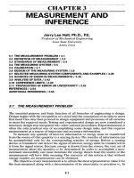
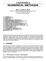
The
considerations necessary
to
accomplish this task
are
illustrated
in
Fig. 3.1.
First,
a

statement
of the
variables
to be
measured along with
their
probable
mag-
nitude,
frequency,
and
other pertinent information must
be
formulated. Next,
one
brings
all the
knowledge
of
fundamentals
to the
measurement problem
at
hand.
This includes
the
applicable electronics, engineering mechanics, thermodynamics,
heat transfer, economics, etc.
One
must have

an
understanding
of the
variable
to be
measured
if an
effective
measurement
is to be
accomplished.
For
example,
if a
heat
flux
is
to be
determined,
one
should understand
the
aspects
of
heat-energy transfer
before
attempting
to
measure
entities

involved with this process.
Once
a
complete understanding
of the
variable
to be
measured
is
obtained
and the
environment
in
which
it is to be
measured
is
understood,
one can
then consider
the
necessary characteristics
of the
components
of the
measurement system. This would
include response, sensitivity, resolution, linearity,
and
precision.
Consideration

of
these
items
then leads
to
selection
of the
individual instrumentation components, including
at
least
the
detector-transducer element,
the
signal-conditioning element,
and a
read-
out
element.
If the
problem
is a
control situation,
a
feedback
transducer would also
be
considered. Once
the
components
are

selected
or
specified, they must
be
coupled
to
form
the
generalized measuring system. Coupling considerations
to
determine
the
iso-
lation characteristics
of the
individual transducer must also
be
made.
Once
the
components
of the
generalized measurement system
are
designed
(specified),
one can
consider
the
calibration technique necessary

to
ensure accuracy
of
the
measuring system.
Energy
can be
transferred into
the
measuring system
by
coupling means
not at
the
input ports
of the
transducer. Thus
all
measuring systems interact with
their
envi-
ronment,
so
that some unwanted signals
are
always present
in the
measuring system.
Such
"noise"

problems must
be
considered
and
either eliminated, minimized,
or
reduced
to an
acceptable level.
If
proper technique
has
been used
to
measure
the
variable
of
interest, then
one
has
accomplished what
is
called
a
valid
measurement. Considerations
of
probability
and

statistics then
can
result
in
determination
of the
precision
or
uncertainty
of the
measurement.
If, in
addition, calculations
of
dependent variables
are to be
made
from
the
measured variables,
one
must consider
how the
uncertainty
in the
mea-
sured
variables propagates
to the
calculated quantity. Appropriate propagation-of-

uncertainty
equations must
be
used
to
accomplish this task.
MEASUREMENT
CALIBRATION PROCEDURE AND/OR
PROBLEM
AND
/*
EQUATIONS
OF
OPERATION
SPECIFICATIONS
|
"-
1
T^
znr
1
.
NOISE
REQUIRED
KNOWLEDGE
OF
FUNDAMENTALS CONSIDERATIONS
ELECTRONICS,
ENGINEERING MECHANICS
I

(i.e.,
STATICS,
DYNAMICS,
STRENGTH
OF
MATERIALS,
AND
FLUIDS),
THERMODYNAMICS,
,
T
,
HEAT TRANSFER
AND
ECONOMICS.
PROPER
LABOR-
[
'
ATORY TECHNIQUE
\
i
INSTRUMENTATION ITEMS
TO
CONSIDER:
I
PROBABILITY
RESPONSE,
SENSITIVITY, RESOLUTION,
\ '

|
CONSIDERATIONS
LINEARITY,
CALIBRATION, PRECISION
I
*
1
REQUIRED,
PHYSICAL CHARACTERISTICS
VALID
I I
OF
THE
ITEM
TO BE
MEASURED SUCH
AS
MEASUREMENT
f
RANGE
OF
AMPLITUDE
AND
FREQUENCY,
'
1
'
STATISTTPAi
ENVIRONMENTAL
FACTORS AFFECTING

ANALYSIS
THE
MEASUREMENT SUCH
AS
TEMPERATURE
]
f
I
"""
1
^
10
VARIATIONS,
ETC.
I
*
1
I
PRECISION
(UNCERTAINTY)
_
1
1
f
OF
MEASUREMENT
^
\
^
SELECTION

OF
I
.
1
.
INSTRUMENTATION
COMPONENTS
VALID
OATA
s
V
ALID
MEASUREMENT
1
PLUS
ITS
ASSOCIATED
PRECISION
(UNCERTAINTY)
»
?
Ir
I
j_
1
DETECTOR
cifiNAL
READOUT
TRANSDUCER
|

CONoSlONING
|
TRANSDUCER
|
J
1
TRANSDUCER
I
CALCULATION
OF
i
i
1
DEPENDENT
VARIABLES
V
»JU
/
i
—-i
1
FEEDBACK
.
1
.
TRANSDUCER
|
PROPAGATION
OF
PRECISION

(UNCERTAINTY
OR
ERROR)
OF
I
'
1
INDEPENDENTLY MEASURED VARIABLES
TO
COUPLING
THE
DEPENDENT CALCULATED QUANTITIES
CONSIDERATIONS
|
j
-
I
GENERALIZEDMEASUREMENTSYSTEM
I
^
™"
'
^nV^JlsIoN
1 1
(UNCERTAINTY)
FIGURE
3.1 The
generalized measurement task.
3.2
DEFINITiON

OF
MEASUREMENT
A
measurement
is the
process
of
comparing
an
unknown quantity with
a
predefined
standard.
For a
measurement
to be
quantitative,
the
predefined standard must
be
accurate
and
reproducible.
The
standard must also
be
accepted
by
international
agreement

for it to be
useful
worldwide.
The
units
of the
measured variable determine
the
standard
to be
used
in the
com-
parison process.
The
particular standard used determines
the
accuracy
of the
mea-
sured variable.
The
measurement
may be
accomplished
by
direct comparison with
the
defined
standard

or by use of an
intermediate reference
or
calibrated system.
The
intermediate reference
or
calibrated system results
in a
less accurate measure-
ment
but is
usually
the
only practical
way of
accomplishing
the
measurement
or
comparison process. Thus
the
factors limiting
any
measurement
are the
accuracy
of
the
unit involved

and its
availability
to the
comparison process through reference
either
to the
standard
or to the
calibrated system.
3.3
STANDARDSOFMEASUREMENT
The
defined standards which currently exist
are a
result
of
historical development,
current practice,
and
international agreement.
The
Systeme
International
d'Unites
(or SI
system)
is an
example
of
such

a
system that
has
been developed through
international agreement
and
subscribed
to by the
standard laboratories throughout
the
world, including
the
National Institute
of
Standards
and
Technology
of the
United States.
The SI
system
of
units consists
of
seven base units,
two
supplemental units,
a
series
of

derived units consistent with
the
base
and
supplementary
units,
and a
series
of
pre-
fixes
for the
formation
of
multiples
and
submultiples
of the
various units
([3.1],
[3.2]).
The
important aspect
of
establishing
a
standard
is
that
it

must
be
defined
in
terms
of
a
physical object
or
device which
can be
established with
the
greatest accuracy
by
the
measuring instruments available.
The
standard
or
base unit
for
measuring
any
physical
entity should also
be
defined
in
terms

of a
physical object
or
phenomenon
which
can be
reproduced
in any
laboratory
in the
world.
Of
the
seven standards, three
are
arbitrarily selected
and
thereafter regarded
as
fundamental
units,
and the
others
are
independently defined units.
The
fundamental
units
are
taken

as
mass, length,
and
time, with
the
idea that
all
other mechanical
parameters
can be
derived
from
these three. These fundamental units were natural
selections because
in the
physical world
one
usually weighs,
determines
dimensions,
or
times various intervals. Electrical parameters require
the
additional specification
of
current.
The
independently defined units
are
temperature, electric current,

the
amount
of a
substance,
and
luminous intensity.
The
definition
of
each
of the
seven
basic units
follows.
At the
time
of the
French Revolution,
the
unit
of
length,
called
a
meter (m),
was
defined
as one
ten-millionth
of the

distance
from
the
earth's
equator
to the
earth's
pole along
the
longitudinal meridian passing through Paris,
France.
This
standard
was
changed
to the
length
of a
standard platinum-iridium
bar
when
it was
discov-
ered that
the
bar's length could
be
assessed more accurately
(to
eight significant dig-

its) than
the
meridian. Today
the
standard meter
is
defined
to be the
length equal
to
1 650
763.73 wavelengths
in a
vacuum
of the
orange-red line
of
krypton isotope
86.
The
unit
of
mass,
called
a
kilogram (kg),
was
originally defined
as the
mass

of a
cubic
decimeter
of
water.
The
standard today
is a
cylinder
of
platinum-iridium alloy
kept
by the
International Bureau
of
Weights
and
Measures
in
Paris.
A
duplicate
with
the
U.S. National Bureau
of
Standards serves
as the
mass standard
for the

United
States. This
is the
sole base unit still
defined
by an
artifact.
Force
is
taken
as a
derived unit
from
Newton's second law.
In the SI
system,
the
unit
of
force
is the
newton
(N), which
is
defined
as
that force which would give
a
kilo-
gram

mass
an
acceleration
of one
meter
per
second
per
second.
The
unit interval
of
time,
called
a
second,
is
defined
as the
duration
of
9192
631770
cycles
of the
radiation associated with
a
specified transition
of the
cesium

133
atom.
The
unit
of
current,
called
the
ampere (A),
is
defined
as
that current
flowing in
two
parallel conductors
of
infinite
length spaced
one
meter apart
and
producing
a
force
of 2 x
10~
7
N per
meter

of
length between
the
conductors.
The
unit
of
luminous
intensity,
called
the
candela,
is
defined
as the
luminous
intensity
of one
six-hundred-thousandth
of a
square meter
of a
radiating cavity
at
the
temperature
of
freezing
platinum (2042
K)

under
a
pressure
of 101 325
N/m
2
.
The
mole
is the
amount
of
substance
of a
system which contains
as
many elemen-
tary
entities
as
there
are
carbon atoms
in
0.012
kg of
carbon
12.
Unlike
the

other standards, temperature
is
more
difficult
to
define
because
it is a
measure
of the
internal energy
of a
substance, which cannot
be
measured directly
but
only
by
relative comparison using
a
third body
or
substance which
has an
observable property that changes directly with temperature.
The
comparison
is
made
by

means
of a
device called
a
thermometer, whose scale
is
based
on the
practi-
cal
international
temperature
scale,
which
is
made
to
agree
as
closely
as
possible with
the
theoretical thermodynamic scale
of
temperature.
The
thermodynamic
scale
of

temperature
is
based
on the
reversible Carnot heat engine
and is an
ideal tempera-
ture scale which does
not
depend
on the
thermometric properties
of the
substance
or
object used
to
measure
the
temperature.
The
practical temperature scale currently used
is
based
on
various
fixed
temper-
ature points along
the

scale
as
well
as
interpolation equations between
the
fixed
temperature points.
The
devices
to be
used between
the
fixed
temperature points
are
also specified between certain
fixed
points
on the
scale.
See
Ref. [3.3]
for a
more
complete discussion
of the
fixed
points used
for the

standards
defining
the
practical
scale
of
temperature.
3
A
THEMEASURINGSYSTEM
A
measuring system
is
made
up of
devices called
transducers.
A
transducer
is
defined
as an
energy-conversion device
[3.4].
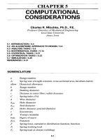
A
configuration
of a
generalized mea-
suring
system

is
illustrated
in
Fig. 3.2.
The
purpose
of the
detector transducer
in the
generalized system
is to
sense
the
quantity
of
interest
and to
transform this information (energy) into
a
form
that will
be
acceptable
by the
signal-conditioning transducer. Similarly,
the
purpose
of the
signal-conditioning
transducer

is to
accept
the
signal
from
the
detector transducer
and
to
modify
this signal
in any way
required
so
that
it
will
be
acceptable
to the
read-
out
transducer.
For
example,
the
signal-conditioning transducer
may be an
amplifier,
an

integrator,
a
differentiator,
or a
filter.
The
purpose
of the
readout transducer
is to
accept
the
signal
from
the
signal-
conditioning transducer
and to
present
an
interpretable output. This output
may be
in
the
form
of an
indicated reading (e.g.,
from
the
dial

of a
pressure gauge),
or it may
be in the
form
of a
strip-chart recording,
or the
output signal
may be
passed
to
either
a
digital processor
or a
controller. With
a
control situation,
the
signal transmitted
to
the
controller
is
compared with
a
desired operating point
or set
point. This compar-

ison dictates whether
or not the
feedback signal
is
propagated through
the
feedback
transducer
to
control
the
source
from
which
the
original signal
was
measured.
An
active
transducer
transforms energy between
its
input
and
output without
the
aid
of an
auxiliary energy source. Common examples

are
thermocouples
and
piezo-
electric crystals.
A
passive
transducer
requires
an
auxiliary energy source (AES)
to
(AES
J
FEEDBACK
I
TRANSDUCER
1
TO
CONTROLLER
I
1 1
JOR
PROCESSOR
\
SOURCE
\
I I
I
1

I
'
1
INDICATOR
J
VARIABLE
1
ncrcr-mo
SIGNAL
ocAnnirr
RECORDER
(
T
0
RF to.
DETECTOR
^
CONDITIONING
to
READOUT
)
MEASURED
^l
TRANSDUCER
p^|
TRANSDUCER
|*J
TRANSDUCER
^-Zlr^
J

T
X
i i
I
(AES
j
f
AES
J
(
AES
J
FIGURE
3.2 The
generalized
measurement system.
AES
indicates auxiliary energy
source,
dashed
line
indicates that
the
item
may not be
needed.
carry
the
input signal through
to the

output. Measuring systems using passive trans-
ducers
for the
detector
element
are
sometimes called
carrier
systems. Examples
of
transducers requiring such
an
auxiliary energy source
are
impedance-based trans-
ducers such
as
strain gauges, resistance thermometers,
and
differential
transformers.
All
impedance-based transducers require auxiliary energy
to
carry
the
information
from
the
input

to the
output
and are
therefore passive transducers.
The
components which make
up a
measuring system
can be
illustrated with
the
ordinary
thermometer,
as
shown
in
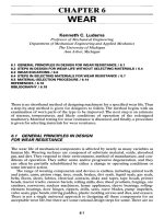
Fig.
3.3.The
thermometric bulb
is the
detector
or
sensing
transducer.
As
heat energy
is
transferred into
the
thermometric bulb,

the
FIGURE
3.3
Components
of a
simple measur-
ing
system.
A,
detector
transducer
(thermometer
bulb with
thermometric
fluid);
B,
signal con-
ditioning stage (amplifier);
C,
readout
stage
(indicator).
thermometric
fluid
(for example, mer-
cury
or
alcohol) expands
into
the

capil-
lary
tube
of the
thermometer. However,
the
small bore
of the
capillary tube pro-
vides
a
signal-conditioning transducer
(in
this case
an
amplifier) which allows
the
expansion
of the
thermometric
fluid
to be
amplified
or
magnified.
The
read-
out in
this case
is the

comparison
of the
length
of the
filament
of
thermometric
fluid
in the
capillary tube with
the
tem-
perature scale etched
on the
stem
of the
thermometer.
Another example
of an
element
of a
measuring
system
is the
Bourdon-tube
pressure gauge.
As
pressure
is
applied

to
the
Bourdon tube
(a
curved tube
of
elliptical cross section),
the
curved tube
tends
to
straighten out.
A
mechanical
linkage
attached
to the end of the
Bour-
don
tube engages
a
gear
of
pinion, which
in
turn
is
attached
to an
indicator needle.

As the
Bourdon tube straightens,
the
mechanical linkage
to the
gear
on the
indicator needle moves, causing
the
gear
and
indicating needle
to
rotate, giving
an
indication
of a
change
in
pressure
on the
dial
of
the
gauge.
The
magnitude
of the
change
in

pressure
is
indicated
by a
pressure scale
marked
on the
face
of the
pressure
gauge.
The
accuracy
of
either
the
temperature measurement
or the
pressure measure-
ment previously indicated depends
on how
accurately each measuring instrument
is
calibrated.
The
values
on the
readout scales
of the
devices

can be
determined
by
means
of
comparison (calibration)
of the
measuring device with
a
predefined stan-
dard
or by a
reference system which
in
turn
has
been calibrated
in
relation
to the
defined
standard.
3.5
CALIBRATION
The
process
of
calibration
is
comparison

of the
reading
or
output
of a
measuring sys-
tem to the
value
of
known inputs
to the
measuring system.
A
complete calibration
of
a
measuring system would consist
of
comparing
the
output
of the
system
to
known
input values over
the
complete range
of
operation

of the
measuring device.
For
example,
the
calibration
of
pressure gauges
is
often
accomplished
by
means
of a
device called
a
dead-weight
tester
where known pressures
are
applied
to the
input
of
the
pressure gauge
and the
output reading
of the
pressure gauge

is
compared
to the
known
input over
the
complete operating range
of the
gauge.
The
type
of
calibration signal should simulate
as
nearly
as
possible
the
type
of
input
signal
to be
measured.
A
measuring system
to be
used
for
measurement

of
dynamic
signals should
be
calibrated using known dynamic input signals. Static,
or
level, calibration signals
are not
proper
for
calibration
of a
dynamic measurement
system because
the
natural dynamic characteristics
of the
measurement system
would
not be
accounted
for
with such
a
calibration.
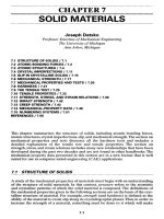
A
typical calibration curve
for a
general transducer
is

depicted
in
Fig. 3.4.
It
might
be
noted that
the
sensitivity
of the
measuring system
can be
obtained
from
the
calibration curve
at any
level
of the
input signal
by
noting
the
relative change
in the
output signal
due to the
relative
change
in the

input signal
at the
operating point.
FIGURE
3.4
Typical calibration curve. Sensitivity
at
//
=
(AO
P
/AI
P
).
TRANSDUCER
3.6
DESIGNOFTHEMEASURINGSYSTEM
The
design
of a
measuring system consists
of
selection
or
specification
of the
trans-
ducers necessary
to
accomplish

the
detection, transmission,
and
indication
of the
desired variable
to be
measured.
The
transducers must
be
connected
to
yield
an
interpretable output
so
that either
an
individual
has an
indication
or
recording
of the
information
or a
controller
or
processor

can
effectively
use the
information
at the
output
of the
measuring system.
To
ensure
that
the
measuring system will perform
the
measurement
of the
specified variable with
the
fidelity
and
accuracy required
of
the
test,
the
sensitivity,
resolution,
range,
and
response

of the
system must
be
known.
In
order
to
determine these items
for the
measurement system,
the
individual trans-
ducer characteristics
and the
loading
effect
between
the
individual transducers
in
the
measuring system must
be
known. Thus
by
knowing individual transducer char-
acteristics,
the
system characteristics
can be

predicted.
If the
individual transducer
characteristics
are not
known,
one
must resort
to
testing
the
complete measuring
system
in
order
to
determine
the
desired characteristics.
The
system characteristics depend
on the
mathematical order (for example,
first-
order, second-order, etc.)
of the
system
as
well
as the

nature
of the
input signal.
If the
measuring system
is a
first-order system,
its
response
will
be
significantly
different
from
that
of a
measuring system that
can be
characterized
as a
second-order system.
Furthermore,
the
response
of an
individual measuring system
of any
order will
be
dependent

on the
type
of
input signal.
For
example,
the
response characteristics
of
either
a
first-
or
second-order system would
be
different
for a
step input signal
and
a
sinusoidal input signal.
3.6.1
Energy
Considerations
In
order
for a
measurement
of any
item

to be
accomplished, energy must move
from
a
source
to the
detector-transducer element. Correspondingly, energy must
flow
from
the
detector-transducer element
to the
signal-conditioning device,
and
energy
must
flow
from
the
signal-conditioning device
to the
readout
device
in
order
for the
measuring system
to
function
to

provide
a
measurement
of any
variable. Energy
can
be
viewed
as
having intensive
and
extensive
or
primary
and
secondary components.
One can
take
the
primary component
of
energy
as the
quantity that
one
desires
to
detect
or
measure. However,

the
primary quantity
is
impossible
to
detect unless
the
secondary component
of
energy accompanies
the
primary component. Thus
a
force
cannot
be
measured without
an
accompanying displacement,
or a
pressure cannot
be
measured without
a
corresponding volume change. Note that
the
units
of the
pri-
mary

component
of
energy multiplied
by the
units
of the
secondary component
of
energy
yield units
of
energy
or
power
(an
energy rate). Figure
3.5
illustrates both
the
active
and
passive types
of
transducers with associated components
of
energy
at the
input
and
output terminals

of
transducers.
In
Fig.
3.5 the
primary component
of
energy
I
p
is the
quantity that
one
desires
to
sense
at the
input
to the
transducer.
A
secondary component
I
s
accompanies
the
primary component,
and
energy must
be

transferred
before
a
measurement
can be
accomplished. This means that pressure
changes
I
p
cannot
be
measured unless
a
corresponding volume change
I
s
occurs.
Likewise, voltage change
I
p
cannot
be
measured unless charges
I
s
are
developed,
and
force
change

I
p
cannot
be
measured unless
a
length change
I
s
occurs. Thus
the
units
of
the
product
I
P
I
S
must always
be
units
of
energy
or
power (energy rate). Some
important transducer characteristics
can now be
defined
in

terms
of the
energy
FIGURE
3.5
Energy
components
for
active
and
passive
transducers.
components shown
in
Fig. 3.5.
These
characteristics
may
have both magnitude
and
direction,
so
that generally
the
characteristics
are
complicated
in
mathematical
nature.

A
more complete discussion
of the
following
characteristics
is
contained
in
Stein
[3-4].
3.6.2
Transducer
Characteristics
Acceptance
ratio
of a
transducer
is
defined
in Eq.
(3.1)
as the
ratio
of the
change
in
the
primary component
of
energy

at the
transducer input
to the
change
in the
sec-
ondary component
at the
transducer input.
It is
similar
to an
input impedance
for a
transducer with electric energy
at its
input:
^=M
^
Emission
ratio
of a
transducer
is
defined
in Eq.
(3.2)
as the
ratio
of the

change
in
the
primary component
of
energy
at the
transducer output
to the
change
in the
sec-
ondary
component
of
energy
at the
transducer output. This
is
similar
to
output
impedance
for a
transducer with electric energy
at its
output:
E
-^
^

AO
S
Transfer
ratio
is
defined
in Eq.
(3.3)
as the
ratio
of the
change
in the
primary com-
ponent
of
energy
at the
transducer output
to the
change
in the
primary component
of
energy
at the
transducer input:
T=^-
(3.3)
A/

p
Several
different
types
of
transfer ratios
may be
defined
which involve
any
out-
put
component
of
energy with
any
input component
of
energy. However,
the
main
transfer
ratio involves
the
primary component
of
energy
at the
output
and the

pri-
mary
component
of
energy
at the
input.
The
main transfer ratio
is
similar
to the
transfer
function,
which
is
defined
as
that
function
describing
the
mathematical
operation that
the
transducer performs
on the
input signal
to
yield

the
output signal
at
some operating point.
The
transfer ratio
at a
given operating point
or
level
of
input
signal
is
also
the
sensitivity
of the
transducer
at
that operating point.
When
two
transducers
are
connected, they
will
interact,
and
energy

will
be
trans-
ferred
from
the
source,
or
first,
transducer
to the
second transducer. When
the
trans-
fer
of
energy
from
the
source transducer
is
zero,
it is
said
to be
isolated
or
unloaded.
ACTIVE
TRANSDUCER

PASSIVE
TRANSDUCER
A
measure
of
isolation
(or
loading)
is
determined
by the
isolation
ratio,
which
is
defined
by
O
p>a
_
O
P>L
^
A
(
.
O
p>i
0
P>NL

A +
\E
S
\
^
'
}
where
a
means actual;
/,
ideal;
L,
loaded;
and NL, no
load.
When
the
emission
ratio
E
s
from
the
source transducer
is
zero,
the
isolation ratio
becomes

unity
and the
transducers
are
isolated.
The
definition
of an
infinite
source
or a
pure
source
is one
that
has an
emission ratio
of
zero.
The
concept
of the
emis-
sion
ratio approaching
zero
is
that
for a
fixed

value
of the
output primary compo-
nent
of
energy
O
p
,
the
secondary component
of
energy
O
8
must
be
allowed
to be as
large
as is
required
to
maintain
the
level
of
O
p
at a

fixed
value.
For
example,
a
pure
voltage source
of 10 V
(O
p
)
must
be
capable
of
supplying
any
number (this
may
approach
infinity)
of
charges
(O
s
)
in
order
to
maintain

a
voltage level
of 10 V.
Like-
wise,
the
pure source
of
force
(O
p
)
must
be
capable
of
undergoing
any
displacement
(O
s
)
required
in
order
to
maintain
the
force level
at a

fixed
value.
Example
1.
The
transfer ratio (measuring-system sensitivity)
of the
measuring sys-
tem
shown
in
Fig.
3.6 is to be
determined
in
terms
of the
individual transducer trans-
fer
ratios
and the
isolation ratios between
the
transducers.
Solution
^
O
3
O
3

O2,L
Q^NL
Ol,L
Ol,L
^
T
r
T
r
j
~
n n n n
i
-
1
^h^2ih^i
M
^2,L
^2,NL
Ui
9
L
^1,NL
i\
=
(product
of
transfer ratios) (product
of
isolation ratios)

3.6.3
Sensitivity
The
sensitivity
is
defined
as the
change
in the
output signal relative
to the
change
in
the
input signal
at an
operating point
k.
Sensitivity
S is
given
by
5
=
lim
№)
=
№)
(3
.5)

A/
P
-»O\
AI
P
//p
=
*
\
dip
Jk
v
'
3.6.4
Resolution
The
resolution
of a
measuring system
is
defined
as the
smallest change
in the
input
signal
that will yield
an
interpretable change
in the

output
of the
measuring system
at
some operating point. Resolution
R is
given
by
R
=
M
p>min
=
^j^-
(3.6)
T,
^l
TRANSDUCER
QI
^
TRANSDUCER
0
^
TRANSDUCER
°3
^
1
**
n
^

n #3
**
FIGURE
3.6
Measuring-system sensitivity.
Example
2. A
pressure transducer
is
to be
made
from
a
spring-loaded piston
in
a
cylinder
and a
dial indicator,
as
shown
in
Fig. 3.7. Known information concern-
ing
each element
is
also listed below:
Pneumatic cylinder
Spring
deflection factor

=
14.28
Ibf/in
= K
Cylinder bore
= 1 in
Piston stroke
=
1
A
in
Dial indicator
Spring
deflector
factor
=
1.22
Ibf/in
= k
Maximum
stroke
of
plunger
=
0.440
in
Indicator dial
has 100
equal divisions
per

360°
Each dial division represents
a
plunger deflection
of
0.001
in
The
following
items
are
determined:
1.
Block diagram
of
measuring system showing
all
components
of
energy (see
Fig.
3.8)
2.
Acceptance ratio
of
pneumatic cylinder:
A
Mp
p FIA K
14.28(16)

_
,

2
^
=
A4
=
V
=
AL
=
^
=
—^
L
=
23
-
lpfflAn
3.
Emission ratio
of
pneumatic cylinder:
£
-=i§:=74=T^8=
0
-
070in/lbf
4.

Transfer
ratio
of
pneumatic cylinder:
A0
p
L LA A K
nncc-
/ •
Tpc
=^=j=^=^=^u^)=^
55m/psl
/
DDF^<NIIRF
I
I^
^
niAi
^
6
S
SQ[JRCE
PL*]
PISTON
-
CYLINDER
\_L+\
SZcATOR
[ZZT
FIGURE

3.8
Pressure-transducer block diagram.
FIGURE
3.7
Pressure transducer
in the
form
of
a
spring-loaded piston
and a
dial indicator.
It can be
determined
by
taking
the
smallest change
in the
output signal
which
would
be
interpretable
(as
decided
by the
observer)
and
dividing

by
the
sensitivity
at
that operating
point.
5.
Acceptance
ratio
of
dial indicator:
^^TT
=
^
=
T"T^
=
a82in/lbf
A/
5
F k
1.22
6.
Transfer ratio
of
dial indicator:
T
01
=
p

=
—
=
(3.6°
per
division)/(0.001
in per
division)
A/p
Lt
=
3600°/in
(or
1000 divisions/in)
7.
Isolation
ratio
between pneumatic cylinder
and
dial indicator:
A
DI
_ Uk _
0.82
_
A
DI
+
Epc
Uk+

1IK
0.82
+
0.07
'
8.
System sensitivity
in
dial divisions
per
psi:
-,
output
DI
output
DI
input
PC
output
input
DI
input
PC
output
PC
input
=
T
DI
IT

PC
=
0.055(0.92I)(IOOO)
-
50.7 divisions/psi
9.
Maximum pressure that
the
measuring system
can
sense:
Maximum
input
=
—^—
x
maximum output
=
—
(440 dial divisions)
= 8.7 psi
10.
Resolution
of the
measuring system
in
psi:
Minimum
input
=

—^—
x
minimum readable output
-
—
(1
dial division)
=
0.02
psi
3.6.5
Response
When time-varying signals
are to be
measured,
the
dynamic response
of the
measur-
ing
system
is of
crucial importance.
The
components
of the
measuring system must
be
selected and/or designed such that they
can

respond
to the
time-varying input signals
in
such
a
manner that
the
input information
is not
lost
in the
measurement process.
Several measures
of
response
are
important
to
know
if one is to
evaluate
a
measuring
system's ability
to
detect
and
reproduce
all the

information
in the
input signal. Some
measures
of
response involve time alone, whereas other measures
of
response
are
more involved. Various measures
of
response
are
defined
in the
following
paragraphs.
Amplitude
response
of a
transducer
is
defined
as the
ability
to
treat
all
input ampli-
tudes

uniformly
[3.5].The
typical amplitude-response curve determined
for
either
an
individual
transducer
or a
complete measuring system
is
depicted
in
Fig. 3.9.
A
typical amplitude-response specification
is as
follows:
^f-
=M±T
I
p
,
min
<I
p
<I
p>max
(3.7)
1

P
The
amplitude-response specification includes
a
nominal magnitude
ratio
M
between output
and
input
of the
transducer measuring system along with
an
allow-
able tolerance
T and a
specification
of the
range
of the
magnitude
of the
primary
input
variable
I
p
over which
the
amplitude ratio

and
tolerance
are
valid.
FIGURE
3.9
Typical
amplitude-response
characteristic.
Frequency
response
can be
defined
as the
ability
of a
transducer
to
treat
all
input
frequencies uniformly [3.5]
and can be
specified
by a
frequency-response curve such
as
that shown
in
Fig. 3.10.

A
typical frequency-response specification would
be the
nominal magnitude ratio
M of
output
to
input signals plus
or
minus some allowable
tolerance
T
specified over
a
frequency range
from
the
low-frequency limit
f
L
to the
high-frequency
limit
f
H
as
follows:
^=M+T
f
L

<f<f
H
(3.8)
1
P
It is the
usual practice
to use the
decibel (dB) rather than
the
actual magnitude
ratio
for the
ordinate
of the
frequency-response curve.
The
decibel,
as
defined
in Eq.
(3.9),
is
used
in
transducers
and
measuring systems
in
specifying frequency

response:
Decibel
=
20
lo
glo
-^-
(3.9)
h
FIGURE 3.10 Typical frequency-response
characteristic.
The
decibel scale allows large gains
or
attenuations
to be
expressed
as
relatively
small
numbers.
Phase
response
can be
defined
as the
ability
of a
transducer
to

treat
all
input-phase
relations uniformly
[3.5].
For a
pure sine wave,
the
phase
shift
would
be a
constant
angle
or a
constant time delay between input
and
output signals. Such
a
constant phase
shift
or
time delay would
not
affect
the
waveform shape
or
amplitude determination
when

viewing
at
least
one
complete cycle
of the
waveform.
For
complex input wave-
forms,
each harmonic
in the
waveform
may be
treated slightly
differently
in the
mea-
suring
system, resulting
in
what
is
known
as
phase
distortion,
as
illustrated
in

Ref.
[3.5].
Response
times
are
valid measures
of
response
of
transducers
and
measuring sys-
tems.
An
understanding
of the
response-time specifications requires that
the
mathe-
matical
order
of the
system
be
known
and
that
the
type
of

input signal
or
forcing
function
be
specified.
Rise time
of a
transducer
or
measuring system
is
defined
for any
order system
subjected
to a
step input.
The
rise
time
is
defined
as
that time
for the
transducer
or
measuring
system

to
respond
from
10 to 90
percent
of the
step-input amplitude
and
is
depicted
in
Fig. 3.11.
Delay time
is
another response time which
is
defined
for any
order system sub-
jected
to a
step input.
The
delay
time
is
defined
to be
that time
for the

transducer
or
measuring
system
to
respond
from
O
to 50
percent
of the
step-input amplitude
and is
depicted
in
Fig. 3.11.
Time constant
is
specifically defined
for a
first-order system subjected
to a
step
input.
The
time constant
T is
defined
as the
time

for the
transducer
or
measuring sys-
tem
to
respond
to
63.2 percent
(or 1 -
e~
l
)
of the
step-input amplitude.
The
time con-
stant
is
specifically illustrated
in
Fig. 3.12, where
the
response
x of the
first-order
system
to
step input
x

s
is
known
to be
exponential
as
follows:
x
=
x
s
(l-e~^)
(3.10)
When
the
time
t is
equal
to the
time constant
T, the
first-order system
has
responded
to
63.2 percent
of the
step-input amplitude.
In a
time span equivalent

to
DELAY
TIME
FIGURE 3.11 Rise time
and
delay time used
as
response times.
INSTRUMENT RESPONSE
STEP
INPUT MAGNITUDE
FIGURE
3.12 Response
of a
first-order
system
to a
step input.
3
time constants,
the
system
has
responded
to
95.0 percent
of the
step-input ampli-
tude,
and in a

time span
of 5
time constants,
the
system
has
responded
to
99.3 per-
cent
of the
step-input amplitude. Thus
for a
first-order system subjected
to a
step
input
to
yield
a
correct reading
of the
input variable,
one
must wait
a
time period
of
at
least

5
time constants
in
order
for the
first-order system
to
respond
sufficiently
to
give
a
correct indication
of the
measured variable.
Transducer
Dynamics. Because
of the
time delay
or
phase
shift
a
transducer
or
measuring
system
may
have,
one

must
be
very
careful
to
ensure that
the
measuring
system
can
respond adequately
if the
input signal
to the
measuring system
is
varying
with
time.
If the
time response
of the
measuring system
is
inadequate,
it may
never
read
the
correct value. Thus

if one
believes
the
output indication
of the
measuring
system
to be a
reproduction
of the
actual value
of the
input (measured) variable
without
understanding
the
dynamics
of how the
measuring system
is
responding
to
the
input signal,
a
crucial error
can be
made.
In
order

to
understand dynamic
response,
one
must recognize that
the
compo-
nents
of the
measuring system have natural physical characteristics
and
that
the
measuring
system
will
tend
to
respond according
to
these natural characteristics
when
perturbed
by any
external disturbance.
In
addition,
the
input signal supplied
to a

transducer
or
measuring system provides
a
forcing
function
for
that trans-
ducer
or
measuring system.
The
equation
of
operation
of a
transducer
is a
differ-
ential equation whose order
is
defined
as the
order
of the
system.
The
response
of
the

system
is
determined
by
solving this
differential
equation
of
operation accord-
ing
to the
type
of
input signal
(forcing
function) supplied
to the
system.
If the
mea-
suring
system
is
modeled
as a
linear system,
the
differential
equation
of

operation
will
be
ordinary
and
linear with constant coefficients. This
is the
type
of
differen-
tial equation that
can be
solved
by
well-known techniques.
The
nature
of the
solu-
tion depends
on the
nature
of the
forcing
function
as
well
as the
nature
of the

physical
components
of the
system.
For
example,
the
thermometric element
of the
temperature-measuring device
can be
modeled
as
shown
in
Fig. 3.13.
For
this
model,
#in
=
<7iost
+
^stored
=
rate
of
heat energy entering control region
FIRST-
ORDER

SYSTEM
and
q
m
=
HA(T
00
-T)
gw
= O
(assumed)
dT
Stored
=
PCV
—
where
A =
surface
area
h =
surface-film
coefficient
of
convective heat transfer
p
=
density
of
thermometric element

c
=
specific
heat capacity
of
thermometric element
T =
temperature
of
thermometric element
t
=
time
The
resulting equation
of the
operation
is
given
as
follows
for the
step input
x
s
=
T
00
-T
0

:
T-T
0
=
(T
00
-
T
0
)(I
-
e-^)
(3.11)
where
T =
pvc/hA.
The
response
x =
T-T
0
is
shown
in
Fig. 3.12.
Another example
of a
first-order system
is the
electric circuit composed

of
resis-
tance
and
capacitive elements
or the
so-called
RC
circuit. Masses
falling
in
viscous
media
also
follow
a
similar exponential characteristic.
If
the
system
is
characterized
by a
second-order linear ordinary
differen-
tial equation,
the
solution becomes
more complex than that
for the

first-
order system.
The
system behavior
depends
on the
amount
of
friction
or
damping
in the
system.
For
example,
the
meter movement
of a
galvanometer
or
D'Arsonval
movement shown
in
Fig.
3.14 such
as
exists
in
many electrical
meters

can be
modeled
as
shown
in
Fig.
3.15. Applying
first
principles
to
this
model yields
the
equation
of
motion
XT
=
J&=T(t)-T
s
-T
f
FIGURE
3.13
Thermometric element
mod-
eled
as a
first-order system.
A,

control region;
B,
thermometric element
at
temperature
T\
C,
envi-
ronment
at
temperature
T
00
.
FIGURE
3.14
D'Arsonval
movement.
A,
spring-retained armature;
B,
field
magnets;
C,
indicating
needle.
FIGURE
3.15
Torques
applied

to the
D'Ar-
sonval
movement.
where
T
s
=
kQ
for
torsional damping
Tf
=
a
6 for
viscous friction
T(t)
=
driving
or
forcing function
Then
/6 +
a9
+ fce
=
T(O
or
e
+

2yco«0
+co^e-^p-
(3.12)
where
CO
n
=
Vfc/7
=
natural undamped frequency
co
rf
=
CO
n
Vl
-
Y^
=
natural damped frequency
COp
=
CO
n
Vl
-
2y
2
=
frequency

at
peak
of
frequency response curve
Y
=
a/G
c
=
damping ratio
a
c
=
V4/c/
=
critical value
of
damping
=
lowest value
of
damping where
no
natural oscillation
of
system
occurs
If
the
damping

is
modeled
as
viscous
friction,
the
possible solutions
to the
equation
of
motion
are
given
by
Eqs.
(3.13),
(3.14),
and
(3.15)
for the
step input.
The
under-
damped solution
of Eq.
(3.12)
is
shown
in
Fig. 3.16.

For
a < 1
(underdamped),
—
=
!-{!-
Y
2
}~
1/2
exp
(-YCO
n
O
sin (GV +
4>)
%s
/T^7
* =
tan-
1
J^
1
J-
(3.13)
For O =
I
(critical
damping),
—

=
!-(!
+
CO
n
O
exp
(-(A
n
t)
(3.14)
X
8
FIGURE
3.16 Response
of a
second-order system
to a
step input.
SECOND-
ORDER
SYSTEM
For
a > 1
(overdamped),
t—(^HwB-^H
'-£$=[
<"
5
>

If
the
system
is
underdamped,
the
response
of the
transducer
or
measuring sys-
tem
overshoots
the
step-input magnitude
and the
corresponding oscillation occurs
with
a
first-order decay. This type
of
response leads
to
additional response specifica-
tions which
may be
used
by
transducer manufacturers. These specifications include
overshoot

OS,
peak time
T
p
,
settling
time
T
5
,
rise
time
T
n
and
delay
time
T
d
as
depicted
in
Fig. 3.16.
If the
viscous damping
is at the
critical value,
the
measuring system
responds

up to the
step-input magnitude only
after
a
very long period
of
time.
If the
damping
is
more than critical,
the
response
of the
measuring system never reaches
a
magnitude
equivalent
to the
step input. Measuring-system components following
a
second-order behavior
are
normally designed and/or selected such that
the
damping
is
less than critical. With underdamping
the
second-order system responds with

some time delay
and a
characteristic phase
shift.
If
the
natural response characteristics
of
each measuring system
are not
known
or
understood,
the
output reading
of the
measurement system
can be
erroneously
interpreted. Figure 3.17 illustrates
the
response
of a
first-order system
to a
square-
wave
input. Note that
the
system with inadequate time response never yields

a
valid
indication
of the
magnitude
of the
step input. Figure 3.18 illustrates
a
first-order sys-
tem
with time constant adequate
(T
«
1//)
to
yield
a
valid indication
of
step-input
magnitude.
Figure 3.19 illustrates
the
response
of an
underdamped second-order
system
to a
square-wave input.
A

valid indication
of the
step-input magnitude
is
obtained
after
the
settling time
has
occurred.
If
the
input
forcing
function
is not a
step input
but a
sinusoidal
function
instead,
the
corresponding
differential
equations
of
motion
to the
first-
and

second-order
systems
are
given
in
Eqs. (3.16)
and
(3.17),
respectively:
x
+ — = A
coseo/f
(3.16)
where
A =
amplitude
of
input signal transformed
to
units
of the
response
variable
derivative(s)
(O/
=
frequency
of
input signal
(forcing

function)
T
=
time constant
FIGURE 3.17
Response
of a
first-order system with
inadequate
response
to a
square-wave
input
(T
>!//).
FIGURE
3.19 Response
of an
underdamped
second-order
system
to a
square
wave.
x
+
2oco«i
+
(tfnx=A
cos

co/£
(3.17)
In
addition,
the
parameters
of the
steady-state responses
of the
first-
and
second-
order system
are
given
by
Eqs.
(3.18)
and
(3.19),
respectively,
and are
shown
in
Figs.
3.20
and
3.21.
The
steady-state solutions

are of the
form
x
ss
= B cos
(co/r
+
0)
where,
for the
first-
and
second-order systems, respectively,
*'
=
v(4y+i
^=-
tan
"
1(
^
(3
-
18)
82
=
V[I
-(coM)
2
]

2
+
(2YCoAo
n
)
2
*
2
=
^
1
1-(4/«I)
2
(319)
From these results
it can be
noted that both
the
first-
and
second-order systems,
when
responding
to
sinusoidal input functions, experience
a
magnitude change
and
a
phase

shift
in
response
to the
input function.
FIGURE
3.18 Response
of a
first-order
system with barely adequate
response
to a
square-wave
input
(T
«
1//).
AMPLITUDE
AMPLITUDE
FIGURE
3.21 Frequency
and
phase response
of a
second-order system
to a
sinusoidal
input.
FIGURE
3.20 Frequency

and
phase response
of a
first-order sys-
tem to a
sinusoidal input.
Many
existing transducers behave according
to
either
a
first-
or
second-order sys-
tem.
One
should understand thoroughly
how
both
first-
and
second-order systems
respond
to
both
the
step input
and
sinusoidal input
in

order
to
understand
how a
transducer
is
likely
to
respond
to
such input signals. Table
3.1 is a
listing
of the
steady-state responses
of
both
the
first-
and
second-order systems
to a
step
function,
ramp
function,
impulse
function,
and
sinusoidal

function.
(See
also [3.6]
and
[3.7].)
Understanding
how a
transducer might respond
to a
complex transient
waveform
can be
understood
by
considering
a
sinusoidal response
of the
system, since
any
complex transient
forcing
function
can be
represented
by a
Fourier series equivalent
[3.5].
Consideration
of

each separate harmonic
in the
input
forcing
function
would
then yield information
as to how the
measuring system
is
likely
to
respond.
Example
3. A
thermistor-type temperature sensor
is
found
to
behave
as a
first-order
system,
and its
experimentally determined time constant
I is 0.4 s. The
resistance-
temperature relation
for the
thermistor

is
given
as
*
=
*oexp[
P
(l-^)]
where
p has
been
experimentally determined
to be
4000
K.
This temperature sensor
is
to be
used
to
measure
the
temperature
of a fluid by
suddenly immersing
the
ther-
mistor into
the fluid
medium.

How
long
one
must wait
to
ensure that
the
thermometer reading
will
be in
error
by
no
more
than
5
percent
of
the
step
change
in
temperature
is
calculated
as
follows:
x
=
x

s
(l
-
e-"*)
x
=
T-T
0
=
Q^(T
00
-T
0
)
x
s
=
T
00
-
T
0
.'.
0.95
=
1 -
e^
A
In
0.05

=
-=^-
=
-2.9957
0.4

t
=
1.198
s = 12 s
Determine
the
sensitivity
of the
thermometer
at a
temperature
of 300 K if the
resistance
R is
1000 ohms
(Q)
at
this temperature:
5
=
^
=*
0
exp[p(i-fY|p(-l)r-

dT
op
\_
\T
TQ)]
=
_R$
=
1000(4000)
T
2
(30O)
2
=
-44.44
Q/K
Determine
the
resolution
of the
thermometer
if one can
observe changes
in
resis-
tance
of
0.50
Q
on a

Wheatstone bridge used
as a
readout device
at the
temperature
of
300
K:
^
=
AQ
l
min=
-^
^
Qon3
K
S
-44.44
TABLE
3.1
Response
of
First-
and
Second-Order Systems
to
Various Input Signals
First-order
system

Second-order
system
Equation
of
Motion
Step input: F(t)
=
F
Impulse
input:
/
Ramp
input:
P(t)
TABLE
3.1
Response
of
First-
and
Second-Order Systems
to
Various Input Signals (Continued)
First-order
system Second-order system
Sinusoidal input: F(t)
=
F
0
cos

Q/
or
F(t)
=
(real part
01)^0
exp
(Kit)
The
expected response
of the
thermometer
if it
were subjected
to
step changes
in
temperature between
300 and 500 K in a
square-wave fashion
and at a
frequency
of
1.0
hertz
(Hz)
is
shown
in
Fig.

3.22, where
x =
x
s
(0.7135). Note that
the
thermistor
never responds
sufficiently
to
give
an
accurate indication
of the
step-amplitude tem-
perature.
However,
if the
time
constant
of the
thermistor
were
selected
to be
less than
0.1 s, the
step-amplitude temperature would
be
indicated

in 0.5 s (5
time constants).
Example
4. A
strip-chart recorder (oscillograph)
has
been determined
to
behave
as
a
second-order system with damping ratio
of 0.5 and
natural
frequency
of 60 Hz.
At
what frequency would
the
output amplitude
of the
recorder
"peak"
even with
a
constant-amplitude input signal?
The
frequency
may be
calculated

as
follows:
co
p
=
CO
n
Vl
-
2y
2
-
60Vl
-
2(0.5)
2
-
42.4
Hz
What
is the
maximum sine-wave frequency
of
input signal that would allow
no
more than
5
percent error
in
amplitude?

See
Fig.
3.23.
The
amplitude factor
(AF)
is
calculated
as
follows:
1.05
=
AF
=
V[l
_
(co//co
^
2]
2
+
(2y
^)
2
=
Vl
_
z
+
Z

2
where
z
=
((0/CO
n
)
2
.
The
result
is
co
/max
=
19.2
Hz.
A
complex waveform made
up of a
fundamental frequency
of 10 Hz and 8
har-
monics
in
terms
of its
Fourier series representation
is
desired

to be
recorded. Will
the
oscillograph described above
suffice?
The
basic equation
is
Maximum
frequency
= (n +
1)
(fundamental)
= 90 Hz
AF
=
—
—
- n 51
V[(l
-
(90/6O)
2
]
2
+
(90/6O)
2
V
=

tan"
1
^°'
/
5
^
/
^
Q
7
=
-55.2°
(oscillograph will
not
suffice)
1
-
(90/60)
If
both
the
frequency
and
phase-response characteristics
for the
oscillograph
are
given
below, show
how the

input signal
to the
oscillograph, also given below, will
be
changed,
and
give
the
resulting relation expected:
e
=
10
+ 5.8 cos 5t + 3.2 cos
1Or
+ 1.8 cos
2Qt
FIGURE
3.22
Thermistor temperature response
of
Example
3.