Sổ tay tiêu chuẩn thiết kế máy P6 ppsx

CHAPTER
4
NUMERICAL
METHODS
Ray
C.
Johnson,
Ph.D.
Higgins
Professor
of
Mechanical
Engineering Emeritus
Worcester
Polytechnic Institute
Worcester,
Massachusetts
4.1
NUMBERS/4.1
4.2
FUNCTIONS
/ 4.3
4.3
SERIES
/ 4.6
4.4
APPROXIMATIONS
AND
ERROR
/ 4.7
4.5

FINITE-DIFFERENCE APPROXIMATIONS
/4.16
4.6
NUMERICAL INTEGRATION
/
4.18
4.7
CURVE FITTING
FOR
PRECISION POINTS
/
4.20
4.8
CURVE FITTING
BY
LEAST SQUARES
/
4.22
4.9
CURVE FITTING
FOR
SEVERAL VARIABLES
/
4.25
4.10 INTERPOLATION
/
4.26
4.11 ROOT FINDING
/
4.28

4.12
SYSTEMS
OF
EQUATIONS
/
4.34
4.13 OPTIMIZATION TECHNIQUES
/
4.37
REFERENCES
/
4.38
In
this chapter some numerical techniques particularly
useful
in the
field
of
machine
design
are
briefly
summarized.
The
presentations
are
directed
toward automated
calculation
applications using electronic calculators

and
digital computers.
The
sequence
of
presentation
is
logically organized
in
accordance with
the
preceding
table
of
contents,
and
emphasis
is
placed
on
useful
equations
and
methods rather
than
on the
derivation
of
theory.
4.1

NUMBERS
In the
design
and
analysis
of
machines
it is
necessary
to
obtain
quantities
for
various
items
of
interest, such
as
dimensions, material properties, area, volume, weight,
stress,
and
deflection. Quantities
for
such items
are
expressed
by
numbers accompa-
nied
by the

units
of
measure
for a
meaningful perspective. Also, numbers always
have
an
algebraic sign, which
is
assumed
to be
positive unless clearly designated
as
negative
by a
minus sign preceding
the
number.
The
various kinds
of
numbers
are
defined
in
Sec. 2-7, which see.
4.1.1 Real
Numbers,
Precision,
and

Rounding
Any
numerical quantity
is
expressed
by a
real
number which
may be
classified
as an
integer,
a
rational number,
or an
irrational number.
For
practical purposes
of
calcu-
lation
or
manufacturing,
it is
often necessary
to
approximate
a
real number
by a

specified
number
of
digits.
For
some cases, significant numbers
may be
useful,
and
the
following
relates
to the
obtainable degree
of
precision.
Degree
of
Precision.
In
machine design, real numbers
are
expressed
by
significant
digits
as
related
to
practical considerations

of
accuracy
in
manufacturing
and
opera-
tion.
For
example,
a
dimension
of a
part
may be
expressed
by
four
significant digits
as
3.876
in,
indicating
for
this number that
the
dimension will
be
controlled
in
man-

ufacturing
by a
tolerance expressed
in
thousandths
of an
inch.
As
another example,
the
weight density
of
steel
may be
used
as
0.283
lbm/in
3
,
indicating
a
level
of
accu-
racy
associated with control
in the
manufacturing
of

steel stock. Both
these
exam-
ples illustrate numbers
as
basic terms
in a
design specification.
However,
it is
often necessary
to
analyze
a
design
for
quantities
of
interest using
equations
of
various types. Generally,
we
wish
to
evaluate
a
dependent variable
by
an

equation expressed
in
terms
of
independent variables.
The
degree
of
precision
obtained
for the
dependent variable depends
on the
accuracy
of the
predominant
term
in the
particular equation,
as
related
to
algebraic operations.
In
what
follows,
we
will
assume that
the

accuracy
of the
computational device
is
better
than
the
num-
ber of
significant
figures
in a
determined value.
For
addition
and
subtraction,
the
predominant term
is the one
with
the
least
number
of
significant decimals.
For
example, suppose
a
dimension

D in a
part
is
determined
by
three machined dimensions
A,
B,
and C
using
the
equation
D=A
+
B-C.
Specifically,
if the
accuracy
of
each dimension
is
indicated
by the
significant
digits
in
A =
12.50
in, B =
1.062

in, and C =
12.375
in, the
predominant term
is A,
since
it has the
least number
of
significant
decimals with only two. Thus
D
would
be
accu-
rate
to
only
two
decimals,
and we
would calculate
D -A + B - C =
12.50
+
1.062
-
12.375
=
1.187

in. We
should then round this value
to two
decimals, giving
D =
1.19
in
as
the
determined value. Also,
we
note that
D is
accurate
to
only three
significant
fig-
ures,
although
A and B
were accurate
to
four
and C was
accurate
to
five.
For
multiplication

and
division,
the
predominant term
is
simply defined
as the
one
with
the
least number
of
significant
digits.
For
example, suppose tensile stress
a
is
to be
calculated
in a
rectangular tensile
bar of
cross section
b by h
using
the
equa-
tion
a =

P/(bh).
Specifically,
if P = 15 000
Ib,
and as
controlled
by
manufacturing
accuracy
b =
0.375
in and h =
1.438
in, the
predominant term
is
b,
since
it has
only
three significant digits. Incidentally,
we
have also assumed that
P is
accurate
to
at
least three
significant
digits. Thus

we
would calculate
a -
P/(bh)
- 15
000/
[0.375(1.438)]
= 27 816
psi.
We
should then round this value
to
three
significant dig-
its,
giving
a = 27 800 psi as the
determined value.
For a
more rigorous approach
to
accuracy
of
dependent variables
as
related
to
error
in
independent variables,

the
theory
of
relative change
may be
applied,
as
explained
in
Sec. 4.4.
Rounding.
In the
preceding examples,
we
note
that
determined
values
are
rounded
to a
certain number
of
significant decimals
or
digits.
For any
case,
the
cal-

culations
are
initially made
to a
higher level
of
accuracy,
but
rounding
is
made
to
give
a
more meaningful answer.
Hence
we
will
briefly
summarize
the
rules
for
rounding
as
follows:
1. If the
least significant digit
is
immediately followed

by any
digit between
5 and 9,
the
least significant digit
is
increased
in
magnitude
by 1. (An
exception
to
this
rule
is the
case where
the
least significant digit
is
even
and it is
immediately
fol-
lowed
by the
digit
5
with
all
trailing zeros.

In
that event,
the
least significant digit
is
left
unchanged.)
2. If the
least significant digit
is
immediately followed
by any
digit between
O and 4,
the
least
significant
digit
is
left
unchanged.
For
example, with three significant digits desired, 2.765
Ol
becomes
2.77,
2.765
becomes
2.76, -1.8743
becomes

-1.87,
-0.4926
becomes
-0.493,
and
0.003
792 8
becomes 0.003
79.
4.1.2
Complex
Numbers
Complex
numbers
are
ones that contain
two
independent parts, which
may be
rep-
resented graphically along
two
independent coordinate axes.
The
independent com-
ponents
are
separated
by
introduction

of the
operator
j =
V^l.
Thus
we
express
complex number
c = a + bj,
where
a and b by
themselves
are
either integers, rational
numbers,
or
irrational numbers. Often
a is
called
the
real
component
and bj is
called
the
imaginary
component.
The
magnitude
for c is VV +

b
2
.
For
example,
if c =
3.152
+
2.683/,
its
magnitude
is
IcI
=
V(3.152)
2
+
(2.683)
2
-
4.139
Algebraically,
the
values
for a and b may be
positive
or
negative,
but the
magnitude

of
c is
always positive.
4.2
FUNCTIONS
Functions
are
mathematical means
for
expressing
a
definite relationship between
variables.
In
numerical applications, generally
the
value
of a
dependent variable
is
determined
for a set of
values
of the
independent variables using
an
appropriate
functional
expression. Functions
may be

expressed
in
various
ways,
by
means
of
tables, curves,
and
equations.
4.2.1
Tables
Tables
are
particularly
useful
for
expressing discrete value relations
in
machine
design.
For
example,
a
catalog
may use a
table
to
summarize
the

dimensions, weight,
basic dynamic capacity,
and
limiting speed
for a
series
of
standard roller bearings.
In
such
a
case,
the
dimensions would
be the
independent variables, whereas
the
weight,
basic
dynamic capacity,
and
limiting speed would
be the
dependent variables.
For
many applications
of
machine design,
a
table

as it
stands
is
sufficient
for
giv-
ing
the
numerical information needed. However,
for
many other applications requir-
ing
automated calculations,
it may be
appropriate
to
transform
at
least some
of the
tabular
data into equations
by
curve-fitting techniques.
For
example,
from
the
tabu-
lar

data
of a
roller-bearing series, equations could
be
derived
for
weight, basic
dynamic
capacity,
and
limiting speed
as
functions
of
bearing dimensions.
The
equa-
tions
would then
be
used
as
part
of a
total equation system
in an
automated design
procedure.
4.2.2
Curves

Curves
are
particularly
useful
in
machine design
for
graphically expressing continu-
ous
relations between variables over
a
certain range
of
practical interest.
For the
case
of
more than
one
independent variable, families
of
curves
may be
presented
on
a
single graph.
In
many cases,
the

graph
may be
simplified
by the use of
dimension-
less
ratios
for the
independent variables.
In
general, curves present
a
valuable pic-
ture
of how a
dependent variable changes
as a
function
of the
independent variables.
For
example,
for a
stepped
shaft
in
pure torsion,
the
stress concentration factor
K

ts
is
generally presented
as a
family
of
curves, showing
how it
varies with
respect
to
the
independent dimensionless variables
rid
and
Did.
For the
stepped
shaft,
r is the
fillet
radius,
d is the
smaller diameter,
and D is the
larger diameter.
For
many applications
of
machine design,

a
graph
as it
stands
may be
sufficient
for
giving
the
numerical data needed. However,
for
many
other
applications requiring
automated calculations, equations valid over
the
range
of
interest
may be
necessary.
The
given graph would then
be
transformed
to an
equation
by
curve-fitting tech-
niques.

For
example,
for the
stepped
shaft
previously mentioned, stress concentration
factor
K
ts
would
be
expressed
by an
equation
as a
function
of r,
d,
and D
derived
from
the
curves
of the
given graph.
The
equation would then
be
used
as

part
of a
total
equation system
in the
decision-making process
of an
automated design
procedure.
4.2.3
Equations
Equations
are the
most
powerful
means
of
function
expression
in
machine design,
especially when automated calculations
are to be
made
in a
decision-making
proce-
dure. Generally, equations express continuous relations between variables, where
a
dependent variable

y is to be
numerically determined
from
values
of
independent
variables
Jc
1
,
Jt
2
,
Jt
3
,
etc. Some commonly used types
of
equations
in
machine design
are
summarized next.
Linear
Equations.
The
general
form
of a
linear equation

is
expressed
as
follows:
y
= b +
C
1
X
1
+
C
2
;c
2
+ - +
c
n
x
n
(4.1)
Constant
b and
coefficient
C
1
,
C
2
, ,

C
n
may be
either positive
or
negative real num-
bers,
and in a
special case,
any one of
these
may be
zero.
For the
case
of one
independent variable
x, the
linear equation
y = b +
ex
is
graph-
ically
a
straight line.
In the
case
of two
independent variables

jti
and
Jt
2
,
the
linear
equation
y = b +
C
1
X
1
+
C
2
Jt
2
is a
plane
on a
three-dimensional coordinate system hav-
ing
orthogonal axes
Jti,
Jt
2
,
and y.
Polynomial

Equations.
The
general
form
of a
polynomial equation
in two
vari-
ables
is
expressed
as
follows:
y
= b +
CiJt
+
C
2
Jt
2
+ - +
c
n
x
n
(4.2)
Constant
b and
coefficients

C
1
,
C
2
, ,
C
n
may be
either positive
or
negative
real
num-
bers,
and in a
special case,
any one of
these
may be
zero.
For the
special case
of n = 1, the
equation
y = b +
C
1
X
is

linear
in x. For the
special
case
of
n = 2, the
equation
y = b +
C
1
X
+
C
2
x
2
is
known
as a
quadratic
equation.
For the
special case
of n = 3, the
equation
y = b +
CiJt
+
C
2

Jt
2
+
C
3
Jt
3
is
known
as a
cubic equa-
tion.
In
general,
for n > 3, Eq.
(4.2)
is
known
as a
polynomial
of
degree
n.
Simple
Exponential
Equations.
The
general
form
for

a
type
of
simple exponential
equation commonly used
in
machine design
is
expressed
as
follows:
y
=
bxpx¥'»x
c
n
»
(4.3)
Coefficient
b and
exponents
C
1
,
C
2
, ,
C
n
may be

either positive
or
negative real
numbers. However, except
for the
special case
of any c/
being
an
integer,
the
corre-
sponding values
of
jc/
must
be
positive.
For the
special case
of
n = 1
with
C
1
=
1,
the
equation
y = bx is a

simple straight line.
For
n
= l
with
C
1
= 2, the
equation
y =
bx
2
is a
simple parabola.
For n = 1
with
C
1
= 3,
the
equation
y =
bx
3
is a
simple cubic equation.
As a
specific example
of the
more general case expressed

by Eq.
(4.3),
a
simple
exponential equation might
be as
follows:
y
2.670
r
2
?
=
38.69-^^
X2
%3
For
this example,
n =
4,
b =
38.69,
C
1
-
2.670,
C
2
=
-0.092,

C
3
=
-1.07,
and
C
4
= 2.
Also,
if
at a
specific
point
we
have
Jt
1
=
4.321,
X
2
=
3.972,
X
3
=
8.706,
and
X
4

=
0.0321,
the
equa-
tion would give
the
value
of
y =
0.1725.
The
general
form
for
another type
of
simple exponential equation occasionally
used
in
machine design
is
expressed
as
follows:
y
=
bc^c
x
2
^c^

(4.4)
Coefficient
b and
independent variables
x
l9
x
2
, ,x
n
may be
either positive
or
neg-
ative real numbers. However, except
for the
special case
of any
x
t
being
an
integer,
the
corresponding values
of
c
t
must
be

positive.
Transcendental
Equations.
The
most commonly encountered types
of
transcen-
dental equations
are
classified
as
being either trigonometric
or
logarithmic.
For
either
case,
inverse
operations
may be
desired.
In
general,
transcendental
equations
determine
a
dependent variable
y
from

the
value
of an
independent variable
x as the
argument.
The
basic trigonometric equations
are y = sin x, y = cos
jc,
and y = tan x. The
argu-
ment
x may be any
real number,
but it
should carry angular units
of
radians
or
degrees.
For
electronic calculators,
the
units
for x are
generally degrees. However,
for
microcomputers
or

larger electronic computers,
the
units
for x are
generally
radians.
The
basic logarithmic equation
is y = log x.
However,
in
numerical applications,
care must
be
exercised
in
recognizing
the
base
for the
logarithmic system used.
For
natural
logarithms,
the
Napierian base
e =
2.718
281 8 is
used,

and the
inverse
operation would
be x =
e
y
.
For
common logarithms,
the
base
10 is
used,
and the
inverse operation would
be x =
10
y
.
A
special relationship
of
importance
is
recognized
by
taking
the
logarithm
of

both sides
in the
simple exponential
Eq.
(4.3), resulting
in the
following
equation:
log y = log b +
C
1
log
X
1
+
C
2
log
X
2
+ - +
C
n
log
X
n
(4.5)
We
see
that this equation

is
analogous
to
linear
Eq.
(4.1)
by
replacing
y,
b,
Jc
1
,
X
2
, ,
X
n
of Eq.
(4.1) with
log y, log
b,
log
Jt
1
,
log
X
2
, ,

log
Jc
n
,
respectively.Thus
the
equa-
tion
y
=
bx
c
will
plot
as a
straight line
on
log-log graph paper, regardless
of the
val-
ues for
constants
b and c.
Combined
Equations. Some basic types
of
equations have
now
been summarized,
and

they
will
be
applied later
in
techniques
of
curve fitting. However,
any of the
more complicated equations
found
in
machine design
may be
considered
as
special
combinations
of the
basic equations, with
the
terms related
by
algebraic operations.
Such
equations might
be
placed
in the
general classification

of
combined equations.
As a
specific
example
of a
combined equation,
a
polynomial equation
is
merely
the
sum of
positive simple exponential terms, each
of
which
has the
general
form
of the
right
side
of
Eq.
(4.3).
4.3
SERIES
A
series
is an

ordered
set of
sequential terms generally connected
by the
algebraic
operations
of
addition
and
subtraction.
The
number
of
terms
can be
either
finite
or
infinite
in
scope.
If the
terms contain independent variables,
the
series
is
really
an
equation
for

calculating
a
dependent variable, such
as the
polynomial
Eq.
(4.2).
If
a
series
is
lengthy,
it is
often
possible
to
approximate
the
series with
a
finite
number
of
terms.
The
criterion
for
determining
how
many terms

of the
sequence
are
necessary
is
based
on a
consideration
of
convergence.
The
number
of
terms used
must
be
sufficient
for
convergence
of the
determined value
to an
acceptable level
of
accuracy
when compared with
the
entire series evaluation. This will
be
considered

specifically
in
Sec.
4.4 on
approximations
and
error.
Some commonly used series
in
machine design
will
be
briefly
summarized next.
A
more complete coverage
can be
found
in any
handbook
on
mathematics,
and
what
follows
is
just
a
small sample.
4.3.1

Binomial
Series
Consider
the
combined equation
y =
(xi+
Jc
2
)",
where
X
1
and
X
2
are
independent vari-
ables
and n is an
integer.
The
binomial series expansion
of
this equation
is as
follows:
y =
(X
1

+
X
2
)"
=
*;
+
«f-^
+
^^*r^
(4.6)
In Eq.
(4.6),
if
integer
n is
positive,
the
series consists
of
n
+1
terms. However,
if
inte-
ger
n is
negative,
in
general

the
number
of
terms
is
infinite
and the
series converges
iixl<xl
4.3.2
Trigonometric
Series
Some
trigonometric relations
will
be
approximated
in
Sec.
4.4
based
on the
series
expansions
summarized
as
follows:
JC
3
X

5
X
1
y
=
sin*
=
*
+

+

(4.7)
y.2
y.4
y.6
y
=
COSX
=
l-^
+
^-^
+

(4.8)
In
Eqs. (4.7)
and
(4.8), angle

x
must
be
expressed
in
radians.
4.3.3
Taylor's
Series
If
any
function
y =
f(x)
is
differentiable,
it may be
expressed
by a
Taylor's series
expansion
as
follows:
y
=/(*)
=/(a)
+
f(a)
^f
1

+
f"(a)
^f^+f'"(a)
&^-
+
-
(4.9)
In Eq.
(4.9),
a is any
feasible
real
number value
of x,
f(a)
is the
value
of
dyldx
at
x
=
a,
f"(d)
is the
value
of
(Pyldx
2
atx

= a, and
f"(d)
is the
value
of
d
3
y/dx
3
at x = a.
If
only
the
first
two
terms
in the
series
of Eq.
(4.9)
are
used,
we
have
a
first-order
Taylor's series expansion
of
f(x)
about

a. If
only
the
first
three terms
in the
series
of
Eq.
(4.9)
are
used,
we
have
a
second-order Taylor's series expansion
of
f(x)
about
a.
If
a = O in Eq.
(4.9),
we
have
the
special case known
as a
Maclaurin's
series expansion

of fo).
4.3.4
Fourier
Series
Any
periodic function
y =
f(x)
= f(x +
2n)
can
generally
be
expressed
as a
Fourier
series expansion
as
follows:
y=fix)
=
v
+ Z
&»
cos
(^)
+
b
«
sin

("*)]
(
41
°)
^
/i
=
i
1
r*
where
«*
=
—
/W
cos
(nx)
dx
for
n
=
0,1,2,3,
(4.11)
K
J
-n
and
&„
=
-

f fix)sin(nx)dx
for
w
-
1,2,3,
(4.12)
Tl
J
-n
Coefficients
a
n
and
£
n
of Eq.
(4.10)
are
determined
by
Eqs.
(4.11)
and
(4.12).
For the
Fourier series expansion
of Eq.
(4.10)
to be
valid,

the
Dirichlet
conditions
summarized
as
follows must
be
satisfied:
1.
f(x) must
be
periodic;
i.e.,
f(x)
=f(x
+
2n)
9
or
f(x -
n)
=f(x
+
n).
2.
f(x) must have
a
single,
finite
value

for any x.
3.
f(x)
can
have only
a
finite number
of
finite
discontinuities
and
points
of
maxima
and
minima
in the
interval
of one
period
of
oscillation.
Techniques
of
numerical integration covered later
can be
applied
to
determine
the

significant Fourier coefficients
a
n
and
b
n
by
Eqs.
(4.11)
and
(4.12), respectively.
A
corresponding finite number
of
terms would then
be
used from
the
Fourier
series
of
Eq.
(4.10)
for
approximating
y
-f(x).
Fourier series
are
particularly valuable when

complex periodic functions expressed graphically
are to be
approximated
by an
equation
for
automated calculation use.
4.4
APPROXIMATIONSANDERROR
In
many applications
of
machine design
and
analysis,
it is
advantageous
to
simplify
equations
by
using approximations
of
various types. Such approximations
are
often
obtained
by
using only
the

significant terms
of a
series expansion
for the
function.
The
approximation used must give
an
acceptable degree
of
accuracy
for the
depen-
dent variable over
the
range
of
interest
for
the
independent variables. After
defining
error next,
we
will summarize some approximations particularly
useful
in
machine
design.
Some other techniques

of
approximation will
be
presented later, under curve
fitting,
interpolation, root
finding,
differentiation,
and
integration.
4.4.1
Error
Relative
error
is
defined
as the
difference
between
an
approximate value
and the
true value, divided
by the
true value
of a
variable,
as in Eq.
(4.13):
e-y-^

(4.13)
From this equation, error
e is
determined
as a
dimensionless decimal,
y
a
is an
approximate value
for
y,
and
y
t
is the
true value
for y. If
y
a
and
y
t
are
expressed
by
equations
as
functions
of an

independent variable
x,
Eq.
(4.13) gives
an
error
equa-
tion
as a
function
of Jt.
Also,
from
Eq.
(4.13)
we see
that error
e
carries
an
algebraic sign.
For
positive
y
t
,
a
positive value
for e
means that algebraically

we
have
the
relation
y
a
>
y
t
,
whereas
for
negative
e we
would have
y
a
<
y
t
.
The
opposite relations
are
true
if
y
t
is
negative.

Finally,
the
magnitude
of
error
is its
absolute value \e\.
For
example,
for
y
a
=
1.003
in and
y
t
=
1.015
in, by Eq.
(4.13)
we
calculate
e =
(1.003
-
1.015)/1.015
=
-0.0118.
This means that

y
a
is
1.18 percent less than
its
true
value
y
t
.
The
magnitude
of the
error
is \e\ =
0.0118.
Incidentally,
if
error occurs
at
random
on two or
more independent variables,
the
accompanying
error
on a
dependent variable
may be
determined statistically. This

will
be
illustrated specifically
by
application
of the
theory
of
variance,
as
presented
later
under relative change.
4.4.2
Arc Sag
Approximation
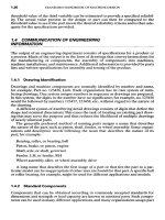
Consider
a
circular
arc of
radius
of
curvature
p as
shown
in
Fig.
4.1
with
sag y

accom-
panying
a
chordal length
of 2x. The
true value
for y can be
calculated
from
the
fol-
lowing
equation
([4.5],
p.
60):
-[>-«]
However,
from
the
right triangle
of
Fig. 4.1,
we
obtain
the
following:
yi=
*±A
If

in
this equation
we
drop
the
term
y
2
t9
the
following approximation
is
derived
for y
(its
use
would obviously
simplify
the
calculation
of
either
sag y or
radius
of
curva-
ture
p):
»
=

£
(4-14)
FIGURE
4.1
Circular
arc of
radius
p
showing
sag y and
chordal
length
2x.
Applying
Eq.
(4.13), error
e in
using approximate
Eq.
(4.14)
is as
follows
([4.5],
p.
62):
e
=
^
=
-sin

2
!
(4.15)
In
Eq.
(4.15), angle
6 is as
shown
in
Fig. 4.1.
As
specific examples,
from
this equation
we
find
that
y
a
by Eq.
(4.14)
has
error
e =
-0.005
for 0 =
8.11°,
e =
-0.010
for

9
=
11.48°,
and e =
-0.02
for
6
=
16.26°. Hence using
the
simple
Eq.
(4.14)
to
calculate
sag
would
be
acceptably accurate
in
many practical applications
of
machine design.
4.4.3
Approximation
for
1/(1
± x)
In
some equations

of
analysis
we
have
a
term
of the
form
(1 + x) in the
denominator.
For
purposes
of
simplification,
as in
operations
of
differentiation
or
integration,
it
may
be
desired
not to
have such
a
term
in the
denominator. Hence consider

the
true
term
y
t
=
1/(1
+
x),
which
can be
expanded into
an
infinite series
by
simple division,
giving
the
following:
»=T77
=1
-*
+
*
2
-*
3
+
-
By

dropping
all but the
first
two
terms
of the
series, 1/(1
+ x) may be
approximated
by
1 -
jc,
expressed
as
follows:
TTT
1
*
=
1
-*
(4
'
16)
Applying
Eq.
(4.13),
the
error
in

using this approximation
is
derived
as
follows:
c
—
y
t
=
(1-JC)-1/(1+JC)
1/(1+Jt)
e
= -x
2
(4.17)
As
specific
examples,
for x
within
the
range
- 0.1
<
x
<
0.1,
we
would have

the
corre-
sponding
error range
of
-0.01
<
e
<
O,
whereas
for
-0.02
<
x
<
0.2 we
would have
-0.04
<
e
<
O.
Hence
a
denominator term
of the
form
1 + x
could

be
replaced
in an
equation
with
a
numerator term
1 -
x,
providing
the
error
is
acceptably small over
the
antici-
pated range
of
variation
for
x.
Similarly,
a
denominator term
of the
form
1 - x
could
be
replaced with

a
numerator term
1 + x if the
error
is
likewise acceptably small.
The
error equation
in
this case would still
be Eq.
(4.17).
4.4.4
Trigonometric
Approximations
Approximations
for
some trigonometric functions will
be
summarized next, fol-
lowed
by the
error
function
as
derived
by Eq.
(4.13)
in
each case.

For the
summa-
rized equations, angle
x
must
be in
radians. However,
in the
examples, ranges
of
angle
x
will
be
given
in
degrees, using
the
notation
x° in
such cases.
An
approximation
for sin x is
obtained
by
using only
the
first
term

in the
Maclau-
rin's series
of Eq.
(4.7)
as
follows:
sin
x
»
x
(4.18)
e
=
-^—-l
(4.19)
sin
x
Hence
for
-10°
<
x°
<
10° we
obtain positive error
for e
with
e
<

0.005
10,
whereas
for
-20°
<
jc°
<
20° we
have positive error
e
<
0.0206.
A
more accurate approximation
for sin x is
obtained
by
using
the
first
two
terms
in
the
series
of Eq.
(4.7)
as
follows:

sin
x
«
*-4-
(4.20)
6
x
{
x
2
\
e
=
-Ml-^H-I
(4.21)
sin
jc
\
6
/
Hence
for
-50°
<
jc°
<
50° we
obtain negative error
for e
with

its
magnitude
Id
<
0.005
41.
An
approximation
for cos x is
obtained
by
using only
the
first
term
in the
Maclau-
rin's series
of Eq.
(4.8)
as
follows:
cosjc-1
(4.22)
e
=
—^ l
(4.23)
COSJC
Hence

for -5°
<
jc°
<
5° we
obtain
positive
error
for
e,
with
e
<
0.003
82,
whereas
for
-15°
<
x°
<
15° we
have positive error
e
<
0.0353.
A
more accurate approximation
for cos x is
obtained

by
using
the
first
two
terms
in
the
series
of Eq.
(4.8)
as
follows:
COSA:
-
1-y
(4.24)
e
=
1
~*
2/2
-I
(4.25)
cos*
Hence
for
-30°
<
x°

<
30° we
obtain negative error
for e
with
its
magnitude
e
<
0.003
58.
An
approximation
for
tan x is
obtained
by
using only
the
first
term
of its
Maclau-
rin's series expansion which
follows:
x
3
2x
5
tan x = x + — +

——
+
—
Thus
the
approximation
and
error
function
are as
follows:
tan
jc
«
x
(4.26)
e
=
-*—-!
(4.27)
tan
x
^
'
Hence
for
-10°
<
x°
<

10° we
obtain negative
error
for e
with
its
magnitude
\e\
<
0.0102.
A
more accurate approximation
for tan x is
obtained
by
using
the
first
two
terms
in
its
series expansion
as
follows:
tan
x
~x
+
Y

(4.28)
x I
x
2
\
e
=
-^-
1+TT
-1
(4.29)
tan*
\
3/
v
'
Hence
for
-30°
<
x°
<
30° we
obtain negative error
for e
with
its
magnitude
\e\
<

0.0103.
4.4.5
Taylor's
Series
Approximations
Consider
a
general differentiable function
y =
/(*).
Its
first-order Taylor's
series
approximation
about
x = a is
obtained
by
using only
the
first
two
terms
of the Eq.
(4.9)
series, resulting
in the
following
equation:
y=f(x)~f(a)

+
(x-a)f(a)
(4.30)
In Eq.
(4.30),
a is any
feasible real number value
of*,
and/'(0)
is the
value
of
dy/dx
at
* = a.
The
accuracy
of Eq.
(4.30) depends
on the
particular
function
/(*)
and the
range
anticipated
for *
about
a. For
this reason,

a
general
error
function
is
difficult
to
derive
and
impractical
to
apply.
The
clue
for
best accuracy
is to
choose
a
value
for a
such
that
(x - a)
will
be
small, resulting
in
negligible terms beyond
the

second
in the
Eq.
(4.9) series.
For
example, suppose
we
consider
f(x)
= sin x and
anticipate
a
range
of
-10°
<
*°
<
10° for
x.
A
good choice
for a
would
be a =
O.
Equation
(4.30) would then give
sin x
~

sin O +
;c
cos O
/.
sin x
~
x
This
is
merely
Eq.
(4.18),
and the
error analysis
for the
anticipated range
of x has
already
been made
after
that equation.
However,
if we
still consider
f(x)
- sin
;c
but
anticipate
a

range
of 45°
<
jc°
<
65°
for
x,
Eq.
(4.18) would
be
highly inaccurate. Hence
Eq.
(4.30) will
be
applied,
and a
good choice
for a
would
be the
midpoint
of the x
range, with
a =
55°(7i/180)
=
0.9599
radian.
Equation (4.30) would then give

the
following approximation:
sin
x
-
sin
0.9599
+
(x
-
0.9599)
cos
0.9599
/.
sin x
-
0.2685
+
0.5736*
Hence
for
x°
= 45° we
would have
y
t
= sin 45° =
0.7071
and
y

a
=
0.2685
+
0.5736(4571/180)
=
0.7190.
For
that value
of*,
the
error
by Eq.
(4.13)
is
-
H!
f^
11
—
For x = 55° we
would have
y
t
= sin 55°
-
0.8192
and
y
a

=
0.2685
+
0.5736(5571/180)
=
0.8191.
For
that value
of
x,
by Eq.
(4.13),
the
error
is
e=
0.8191
8
-a8192
=
_
00001
Finally,
for x = 65° we
would have
y
t
= sin 65°
-
0.9063

and
y
a
=
0.2685
+
0.5736(6571/180)
=
0.9192.
For
that value
of
x,
by Eq.
(4.13),
the
error
is
-^fsIP—
For any
differentiable
/(;c),
a
more accurate approximation
can be
obtained
by
using
the
first

three terms
of the Eq.
(4.9) series, giving
a
second-order Taylor's
series
approximation
about
x = a. The
technique
is
similar
to
what
has
been illustrated
for
a
first-order
Taylor's series approximation.
An
appreciably greater range
of
accuracy
would
be
achieved
at the
expense
of

increased complexity
for the
approximation
derived.
4.4.6
Fourier
Series
Approximation
The
Fourier series
of Eq.
(4.10) involves
an
infinite number
of
terms,
and for
practi-
cal
calculations, only
the
significant ones should
be
used.
The
clue
for
significance
is
the

relative magnitude
of a
Fourier
coefficient
a
n
or
b
n
,
since
the
amplitudes
of sin nx
and
cos nx in Eq.
(4.10)
are
both unity regardless
of
n.
In
establishing significance
of a
Fourier coefficient,
Eqs.
(4.11)
and
(4.12)
are

solved,
perhaps automatically
by a
computer using numerical integration.
The
Fourier
coefficients
are
determined
for n =
1,2,3, ,
N,
where generally
a
value
of
N
equal
to 10 or 12 is
sufficient
for the
investigation. Only
the
coefficients
of
signif-
icant relative magnitude
for
a
n

and
b
n
are
retained. They determine
the
significant
harmonic content
of the
periodic
function
/(*),
and
only
those
coefficients
are
used
in
the Eq.
(4.10) series
for the
approximation derived.
An
error analysis could then
be
made
for the
derived approximation, including perhaps
a

graphic presentation
by
a
computer video display
for
comparative purposes.
As a
final
item
of
practical importance,
a
Fourier series approximation
can be
derived
for
many nonperiodic
functions/(x)
if
independent variable
x is
limited
to a
definite
range corresponding
to
2ft.
In
such
a

case,
the
derived approximation
is
used
for
calculation purposes only within
the
confined range
for x.
Hence
the
derivation
assumes
hypothetical periodicity outside
the
confined
x
range.
Of
course,
the
Dirich-
let
conditions previously stated must
be
satisfied
for/(x)
within that range.
4.4.7

Relative
Change
and
Error
Analysis
Consider
a
general
differentiable
function expressed
as
follows
and
used specifically
for
calculating dependent variable
y in
terms
of
independent variables
X
15
X
2
,
,X
n
:
y=
/(X

1
,
X
29
,X
n
)
(4.31)
By
the
theory
of
differentiation,
we can
write
the
following equation
in
terms
of
par-
tial
derivatives
and
differentials
for the
variables:
dy
=
-J^dX

1
+
^-dx
2
+ - +
^dX
n
(4.32)
d*i
dx
2
dx
n
Small
changes
Ax
1
,
Ax
2
, ,
Ax
n
in
Jt
1
,
X
2
, ,

X
n
can be
substituted respectively
for
the
differentials
dxi,
dx
2
, ,
dx
n
of Eq.
(4.32).Thus
we
obtain
an
approximation
for
estimating
the
corresponding change
in y,
designated
as Ay in the
following equa-
tion:
*-£*"•*£***-*£*
<«

3
>
This
equation
can be
used
to
estimate
the
change
in y
corresponding
to
small
changes
or
errors
in
X
1
,
Jt
2
, ,
Jc
n
.
As an
example
of

application
for Eq.
(4.33), consider
the
simple exponential
Eq.
(4.3),
since many equations
in
machine design
are of
this general
form.
Application
of
Eq.
(4.33)
to Eq.
(4.3) results
in the
following
simple approximation
([4.5],
pp.
67-69):
Ay
Ax
1
Ax
2

Ax
n
-*-
«
C
1
+
C
2
+ - +
C
n
(4.34)
y
X
1
X
2
n
X
n
^
J
In
this equation
byIy,
Ax^x
1
,
Ax

2
/X
2
, ,
Ax
n
/X
n
are
dimensionless ratios corre-
sponding
to
relative changes
in the
variables
of Eq.
(4.3).
As a
specific
example
of
application
for Eq.
(4.34), suppose
we are
given
the
fol-
lowing
simple exponential equation:

c
09
r
1.62
y
2
y-^jk*-
(4-35)
X
2
If
at a
point
of
interest
we
have
the
theoretical
values
X
1
=
3.796,
X
2
=
1.095,
and
X

3
=
2.543, then
Eq.
(4.35) results
in a
theoretical value
of
y =
230.35. Suppose that
errors exist
on the
theoretical values
of
X
1
,
X
2
, ,
X
n
,
specifically given
as
Ax
1
=
0.005,
AjC

2
=
0.010,
and
AjC
3
=
-0.020.
By Eq.
(4.34)
we
calculate
the
corresponding
relative change
in y of Eq.
(4.35)
as
follows:
Au^m^m^.^
Thus
the
given errors
AjC
1
,
Ax
2
, ,
Ax

n
would result
in a
corresponding error
of
Ay
-
-0.0397(230.35)
=
-9.14
on the
theoretical value
of
y =
230.35.
In
the
manner illustrated
by the
preceding example,
by
application
of Eq.
(4.34),
accuracy
estimates
can
quickly
be
made

for
simple exponential equations
of the Eq.
(4.3)
form.
The
worst possible combination
of
errors
for
AjC
1
,
AJt
2
, ,
Ax
n
can be
used
to
estimate
the
corresponding error
Ay on the
theoretical value
for y.
However,
for
cases where random errors

are
anticipated
on the
independent variables,
a
sta-
tistical
approach
is
more appropriate. This will
be
considered next.
A
Statistical
Approach
to
Error
Analysis.
Consider
a
general
differentiable
func-
tion
of
several variables typically expressed
by Eq.
(4.31).
Suppose that relatively
small

errors
are
anticipated
on the
theoretical values
of the
independent variables
JCi,
JC
2
, ,
Jc
n
,
with
a
normal distribution
of
relatively small spread
on any
theoretical
value
for
each variable considered
as the
mean. Designate
the
standard deviation
of
the

normal distribution
for
each variable respectively
by
C^
1
,
C^
2
, ,
&
Xn
.
Then,
for
most
cases, dependent variable
y
would approximately have
a
corresponding normal
distribution
with standard deviation
oy
on its
theoretical value.
«#-(%№*(£!<»•?+-+(£}«'•*
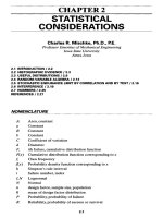
<436)
Suppose
each

of the
independent
variables
Jc
1
,
Jc
2
, ,
jc
n
has a
normal distribu-
tion
typically shown
in
Fig.
4.2
with
theoretical
value
corresponding
to the
mean
value
X
1
for
variable
jc/.

Let
AJC/
represent
a
tolerance
band,
as
shown
in
Fig. 4.2, cor-
responding
to,
say,
three
standard deviations.
If the
tolerance
band
Ax
t
corresponds
to
three
standard deviations, 99.73
percent
of the
total
population
for
x

t
values would
be
within
the
range
jc/
-
AJC/
<
Jc
1
-
+
AJC/,
and we
would
use the
following
relation:
AXi
=
3(5
xi
for/
=
1,2,
,/i
(4.37)
Combining

Eq.
(4.37) with
Eq.
(4.36)
by
eliminating
a*,
for i =
1,2, ,
n,
and
using
the
corresponding
relation
Ay =
3o
y
,
we
obtain
the
following:
(Ay)*
-
(^)W.)
2
+
(J^W
+

"
+
(^)W
(438)
\
CCC
1
/
\
CfJC
2
/
\
ox
n
)
In
this
equation,
all the
tolerance
bands
Ay,
AJCI,
AjC
2
, ,
AjC
n
would

correspond
to
three
standard
deviations
and
would
encompass
99.73
percent
of the
total
popula-
tion
for
each variable.
As an
example
of
application
of Eq.
(4.38),
we
will
consider
the
general
linear
equation
expressed

by Eq.
(4.1).
Hence
by
calculus
we
obtain
3y/3jc
1
=
C
1
,
3y/3jc
2
=
C
2
, ,
3y/3jc«
=
c
n
.
Substituting
these
relations
in Eq.
(4.38),
we

obtain
the
following
approximation
for use in the
case
of
linear
Eq.
(4.1):
(Ay)
2
«
(C
1
AJC
1
)
2
+
(C
2
AjC
2
)
2
+
-
+
(c

n
Ajc«)
2
(4.39)
FIGURE
4.2
Typical normal distribution curve
for an
independent variable
X
1
.
As a
specific example, suppose
we
have
the
following linear
equation:
y
=
2.9Ix
1
-
3.42x
2
+
7.8Ix
3
If

tolerances
of
AjC
1
=
±0.005,
AJt
2
=
±0.015,
and
Ax
3
=
±0.010 exist
on the
theoretical
values
of
^
1
,
Jc
2
,
and
Jt
3
,
we

calculate
the
corresponding tolerance
Ay on the
theoreti-
cal
value
of
y
statistically
by Eq.
(4.39)
as
follows:
(Ay)
2
-
[2.97(0.005)]
2
+
[-3.42(0.015)]
2
+
[7.81(0.01O)]
2
/.
Ay
«
±0.0946
Thus

the
theoretical value
of y
calculated
by the
given linear equation would have
a
corresponding tolerance
of Ay
~
±0.0946.
All the
tolerances would correspond
to,
say,
three standard deviations.
As
another example
of
application
for Eq.
(4.38),
we
will consider
the
general
simple
exponential equation expressed
by Eq.
(4.3).

By
application
of
calculus
to
Eq.
(4.3),
we
obtain
the
expressions
for
dy/dxi,
dy/dx
2
, ,
dy/dx
n
,
which
are
then
substituted
into
Eq.
(4.38). Dividing
the
left
and
right sides

of
this equation, respec-
tively,
by the
left
and
right
sides
of Eq.
(4.3),
we
obtain
the
following approximation
for
use in the
case
of
simple exponential
Eq.
(4.3):
/A
1
V
^
/C
1
A^V
+
/C

2
A^
1
V
+
+
/C
2
A^V
\y I
\
X
1
/
\
X
2
/
\
X
n
)
As a
specific
example, suppose
we are
given
the
same simple exponential equa-
tion

as
before
in Eq.
(4.35).
At a
point
of
interest,
we
have
the
same theoretical val-
ues as
before
for
Jt
1
,
Jc
2
, ,
x
n
and y, and
they
are
given
following
Eq.
(4.35).

However,
the
tolerance bands
are now
given
as
A#i
=
±0.005,
A
Jt
2
=
±0.010,
and
AjC
3
=
±0.020,
all
corresponding
to
three standard deviations. Using
the
stated values fol-
lowing
Eq.
(4.40),
we
calculate statistically

the
corresponding tolerance
Ay on the
theoretical value
of y as
follows:
MlL-Y
~
[
1-62(0.005)f
r-2.86(0.01Q)1
2
[2(0.02O)]
2
\230.35/
[
3.796
J
|_
1.095
J [
2.543
J
"
>'~-'-
u
Thus
the
theoretical value
of y

calculated
by Eq.
(4.35)
as y =
230.35 would have
a
tolerance
of
Ay
~
±7.04, corresponding
to
three standard deviations.
As a
final
note,
based
on the
given possibilities,
we
calculated
Ay
«
-9.47
in the
example following
Eq.
(4.35). However, based
on
probabilities,

we
have calculated
Ay
~
±7.04
in the
present example.
4.5
FINITE-DIFFERENCE
APPROXIMATIONS
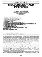
Consider
the
general
differentiable
function
y =
f(x)
graphically shown
in
Fig. 4.3.
First
and
second derivatives
can be
approximated
at a
point
k
of
interest

by the
application
of
finite-difference
equations.
The
simplest
finite-difference
approxima-
tions
are
summarized
as
follows
([4.5],
pp.
28-35):
FIGURE
4.3
Graph
of
y
=f(x)
showing
three successive points used
in
finite
difference
equations.
(&-}

,**'-*-'
(4.4i)
\dx)
k
2A*
v
'
(^y_\
yk-i+y
k
+
i-2y
k
(442}
U
2
Jr
(A*)
2
(442)
Equations (4.41)
and
(4.42) approximate
the
first
and
second derivatives
of y
with
respect

to x,
respectively,
at x =
x
k
.
For
both equations,
the
point
of
interest
at
x
k
is
surrounded
by two
equally spaced points,
at
x
k
_
i
and
x
k
+1.
The
equal increment

of
spacing
is
AJC.
The
values
of
y
=f(x)
at the
three successive points
x
k
_
l9
x
k
,
and
x
k
+1
are
y
k
-i,y
k
,
and
y

k
+19
respectively.
For
most
differentiable
functions
y =
/(jc),
the
given
finite-difference
equations
are
reasonably accurate
if the
following
two
conditions
are
satisfied:
1.
Spacing increment
Ax,
in
general, should
be
reasonably small.
2. The
values

for
y
k
_
l5
y
k
,
and
y
k
+
1
must carry enough significant
figures
to
give
acceptable accuracy
in the
difference
terms
of
Eqs. (4.41)
and
(4.42).
Adequate smallness
of
AJC
can be
determined

by
trial, that
is, by
successively
decreasing
A*
until
no
significant
difference
is
determined
in the
calculated deriva-
tives.
As a
very simple test example, consider
the
function
y = sin
jc.
Suppose
we
wish
to
calculate
first
and
second derivatives
at

x
k
= 35°
using Eqs. (4.41)
and
(4.42).
We
arbitrarily choose
the
increment
AJC°
= 2°,
giving
jc?
_
i
= 33° and
jc?
+1
=
37°. Thus
y
k
_!
= sin 33° =
0.544 639,
y
k
= sin 35° =
0.573 576,

and
y
k
+
1
=
sin 37° =
0.601 815.
However,
for
Eqs. (4.41)
and
(4.42), increment
AJC
must
be
expressed
in
radians, giv-
ing
AJC
=
2(71/180)
=
0.034
906 6
radian.
Hence
by Eq.
(4.41)

we
calculate
/
dv_\
^
0.601815-0.544639
\dx)
k
2
AJC
=
0.057176
"
2(0.0349066)
-
0.818
99
Also,
by Eq.
(4.42),
we
calculate
(d
2
y\
_
0.544
639 +
0.601
815

-2(0.573
576)
(djf
)
k
"
(A*)*
_
Q.QOQ
698
~
(0.034
906
6)
2
=
-0.573
To
check
the
accuracy
of the
approximations,
for y - sin
jc
we
know
by
calculus that
dy/dx

= cos
jc
and
d
2
y/dx
2
=
-sin
x.
Therefore,
the
theoretically correct derivatives
are
calculated
as
(dyldx\
=
cos
jc
= cos 35° =
0.819
15 and
(d
2
y/dx
2
)
k
=

-sin
jc
=
-sin
35° =
-0.5736.
We see
that
the
finite-difference
approximations were reasonably accurate,
which
could
be
further
improved
by
reducing
AJC°
to,
say,
1°.
Finite-difference
approximations
can
also
be
used
for
solving

differential
equa-
tions.
Equations (4.41)
and
(4.42)
can be
used
to
substitute
for
derivatives
in
such
differential
equations, also substituting
jc
=
jc^
where encountered.
The
range
of
inter-
est for x is
divided into small increments
Ax. At
each
net
point

so
obtained,
the
finite-difference-transformed
differential
equation
is
evaluated
to
determine
the
discrepancies
of
satisfaction, known
as
residuals.
An
iterative procedure
is
logically
developed
for
successively relaxing
the
residuals
by
changing
x
values
at the net

points until
the
differential
equation
is
approximately satisfied
at
each
net
point.
Thus
the
solution
function
y =
f(x)
is
approximated
at
each
net
point
by
such
a
numerical technique.
The
iterative procedure
of
relaxation

is
greatly facilitated
by
using
a
digital computer.
As a
final
item,
finite-difference
Eqs. (4.41)
and
(4.42)
may be
applied
to
calcu-
late partial derivatives
for the
case
of a
differentiable
function
of
several variables.
Hence,
for the
equation
y =
/(XI,

Jt
2
,
,*/, ,
X
n
),
the
first
and
second partial
derivatives
may be
approximated
as
follows:
(^)
-
0
^:*-
0
'
(4-43)
\dxij
k
2Ax
1
(Q)
-<*-
1+

y^"
2
*>'
(4.44)
\dx
2
J
k
(AJC
1
-)
2
In
these equations,
the
difference
terms
are
subscripted
by i,
indicating that only
X
1
is
incremented
by
Ax
1
-
for

calculating
y
k
_
1
and
y
k
+
1?
holding
the
other independent
variables
Jt
1
,
Jt
2
,
,Jt
n
constant
at
their
k
point values.
4.6
NUMERICALINTEGRATION
Often

it is
necessary
to
evaluate
a
definite integral
of the
following
form,
where
y =
f(x)
is a
general integrand
function:
I=l"ydx
(4.45)
XQ
For the
case where
y =
f(x)
is a
complicated
function,
numerical integration will
greatly
facilitate obtaining
the
solution.

If
software
is
available
for a
particular com-
putational device,
the
program should
be
directly applied. However,
a
commonly
used numerical technique will
be
described next
as the
basis
for
writing
a
special
program
if
necessary.
A
simple
and
generally very accurate technique
for

numerical integration
is
based
on
Simpson's rule, referring
to
Fig.
4.4 for
what
follows.
First,
the
limit range
for
Jt,
between
Jt
0
and
x
n9
is
divided into
n
equal intervals
by Eq.
(4.46), where
n
must
be an

even number:
Ajc=
**-*o
^
446
)
The
values
of
y
are
then calculated
at
each
of the net
points
so
determined, giving
^
0
,
3>i»3>2»
• •
•,
y
n
-
2,
y
n

-1,3V
Simpson's rule, given
by Eq.
(4.47),
is
then used
to
approx-
imate
the
definite
integral
/ of Eq.
(4.45):
J
~
-f-
l(yo
+
yn)
+
4(3>i
+
3>3
+ - +
J
n
-i)
+
2(y

2
+
y,
+
-
+
y
n
_
2
)]
(4.47)
FIGURE
4.4
Graph
of y =
f(x)
divided
into
equal
increments
for
numerical
integration
between
XQ
and
Jc
n
by

Simpson's
rule.
With
automated computation being used, probably
the
simplest
way for
determining
adequacy
of
smallness
for Ax is by
trial.
Hence
even integer
n is
successively
increased until
the
difference
between successive
7
calculations
is
found
to be
negli-
gible.
As a
very simple test example, consider

the
following
definite integral:
I=I
sin x dx
XQ
Suppose
the
limits
of
integration
are
XQ
= 30° and
x°
=
60°, giving
y
0
= sin 30° and
y
n
= sin
60°.
For the
test example,
a
value
of n = 20 is
arbitrarily chosen. Equation

(4.46)
is
used
to
calculate
AJC
as
follows,
which must
be
expressed
in
radians
for use
in
Eq.
(4.47):
A,
=
M^/1M
=
0.0261799388
In
degrees,
the
increment
is
AJC°
= (60 -
30)/20

=
1.5°.
The y
values
at the
remaining
net
points
are
then calculated
as
y
1
= sin
31.5°,
y
2
= sin
33°, ,
y
n
_
2
= sin
57°,
and
y
n
-1
= sin

58.5°. Simpson's rule
is
then applied using
Eq.
(4.47)
to
calculate
the
approximate value
of
/
=
0.366
025 404 7. The
described procedure,
of
course,
is
pro-
grammed
for
automatic calculation,
and
specifically
the
TI-59
Master Library
Pro-
NET
POINTS

gram
ML-09
was
used
for the
test example
[4.11].
To
check
the
accuracy
of the
approximation,
from
elementary calculus
we
know that
Jsin
x dx is
-cos
x.
Hence,
theoretically,
we
obtain
/=
[(-cos
60°)
-
(-cos

30°)]
=
0.366
025 403 8, and we see
that
the
approximation
for
7
by
Simpson's rule
was
extremely accurate.
See
Sec.
5.4 for
Richardson's error
estimate
when area
is not
known.
4.7
CURVE FITTING
FOR
PRECISION POINTS
Consider
the
situation where
we
have corresponding values

of x and y
available
for
a
finite
number
of
data points. Suppose
we
wish
to
derive
an
equation which passes
precisely through some
or all of
these given data sets,
and
these
we
will
call
precision
points.
Some techniques
of
curve
fitting
for
precision points

will
now be
presented.
In
each case, accuracy checks could
be
made
for the
derived equation relative
to all
the
given data points. Validity
of the
equation over
the
range
of
interest could then
be
established.
4.7.1
Simple Exponential Equation
Curve
Fit
In
many cases
of
machine design, given graphs
or
tabular data would plot approxi-

mately
as a
straight line
on
log-log graph paper. Stress concentration factor graphs
and
a
table
of
tensile strength versus wire diameter
for
spring steel
are
good exam-
ples.
In
such cases,
a
simple exponential equation
of the
following
form
can
readily
be
derived
for
passing through
two
precision points

(it is
assumed that both
x and y
are
positive):
y
=
bx
c
(4.48)
General curve shapes which
are
compatible with
Eq.
(4.48)
are
summarized graphi-
cally
in
Fig.
2.4 of
Ref.
[4.5].
Taking
the
logarithm
of
both sides
in Eq.
(4.48) results

in
the
following,
which reveals that
a
straight line would
be the
plot
on
log-log graph
paper:
log y = c log x + log b
(4.49)
Suppose
two
precision points
(Jc
1
,
^
1
)
and
(x
2
,y
2
)
are
chosen

from
the
given data
sets.
The
algebraic order
for x is
X
1
<
X
2
.
If we use
these precision points
in Eq.
(4.49),
we
obtain
the
following:
log
y
1
= c log
XI
+ log b
log
y
2

= c log
X
2
+ log b
Subtracting
the
preceding
two
equations gives
the
following
relation
for
calculating
exponent
c:
C
=
^M_
(450)
log
(X
2
Ix
1
)
Either
one of the two
precision points
can

then
be
used
to
calculate
coefficient
b as
follows,
as
derived
from
Eq.
(4.48):
*
=
"
(4.51)
X
1
X
2
With
values
of c and b so
determined,
the
simple exponential equation
is
uniquely
defined.

As a
simple example, suppose
we
have available
the
following data
for two
pre-
cision points:
_*
y_
0.1 8.5
0.25
5.3
Equation (4.50) would then yield
the
following value
for
exponent
c:
log
(5.3/8.5)
.
c
=
_
Q516
log
(0.25/0.1)
Equation (4.51) would then give

the
following
value
for
coefficient
b:
*=(d^=
2
-
591
Therefore,
the
derived equation passing through
the
given precision points
is as
follows:
2.591
y ~
^0.516
Accuracy checks could then
be
made using
Eq.
(4.13)
for all
known data points
to
determine
the

validity
of the
derived equation over
the
range
of
interest.
4.7.2
Polynomial Equation
Curve
Fit
A
polynomial equation
of the
following
form
can be
derived
to
pass through
(n + 1)
given
precision points:
y
= b +
CIA:
+
C
2
*

2
+
•••
+
c
n
x
n
(4.2)
The (n + 1)
given data sets
are
substituted into
Eq.
(4.2), giving
(n + 1)
linear equa-
tions
in
terms
of
b,
Ci,
C
2
, ,
C
n
.
These

(n
+1)
linear equations
are
then solved simul-
taneously
for the (n + 1)
unknowns
b,
C
1
,
C
2
, ,
C
n
,
which uniquely defines
the
polynomial
equation.
As a
simple example, suppose
we
wish
to
derive
a
polynomial equation through

the
following
four
precision points. With
(n + 1) = 4, we
will obtain
a
polynomial
equation
of the
third degree, since
n = 3.
_*
y_
0.0 2.0
0.1
1.65
0.2
1.50
0.3
1.41
Substituting
these
data sets into
Eq.
(4.2),
we
obtain
the
following:

2.0 = b
/.1.65
= 2.0 +
C
1
(O.!)
+
C
2
(O.!)
2
+
C
3
(O.!)
3
1.50
-
2.0 +
d(0.2)
+
c
2
(0.2)
2
+
c
3
(0.2)
3

1.41
= 2.0
+C
1
(OJ)+
c
2
(0.3)
2
+
c
3
(0.3)
3
Simultaneous solution
of
these linear equations gives
b =
2.0,
C
1
=
-4.97,
C
2
=
17.0,
and
C
3

=
-23.3.
Therefore,
the
derived polynomial equation passing through
the
four
pre-
cision points
is as
follows:
y
=
2.0
-
4.97*
+
17.0*
2
-
23.3*
3
Accuracy checks could then
be
made using
Eq.
(4.13)
for all
known data points
to

determine
the
validity
of the
derived equation over
the
range
of
interest.
4.8
CURVE FITTING
BY
LEAST SQUARES
In
many cases
of
machine design
we
wish
to
derive
a
simple equation
y =
f(x)
which
approximates
a
large number
of

given data points
(x
k
,
y
k
)
for k =
1,2, ,
M, as
illus-
trated
in the
following table:
*
y_
XI
yi
X
2
)>2
x
k
yk
XM
yu
The
given data points
are
illustrated

by +
symbols
in
Fig. 4.5, which also shows
the
curve
of the
equation
y
=f(x)
to be
derived.
For any
x
k
,
the
difference between
the
given
point value
y
k
and the
corresponding equation value
f(x
k
)
is
Ay^,

defined
as
follows:
Ay*
=
y*-/(**)
(4.52)
The
equation
y
=f(x)
which minimizes
the
summation
of
(Ay
^)
2
terms
for k = 1 to M
of
the
given data
set is
known
as the
least-squares
fit.
A
measure

of
accuracy
for the
derived
equation
is
given
by the
dimensionless correlation coefficient
r,
which will
have
a
value close
to
unity
for the
case
of a
"good"
fit. Some simple examples will
now
be
summarized
for use in
special cases
of
programming, although software pro-
grams
are

often
already available
for
direct application
[4.11].
FIGURE
4.5
Least-squares curves
y =
f(x)
for
given data points indicated
by +.
4.8.1
Linear
Equation
Fit
f
Consider
the
equation
of a
straight line
as
follows, which
is to be
used
for
curve fit-
ting

in the
case where
the
given
set of
data points approximates
a
straight line
on a
graph:
y
= b +
ex
(4.53)
Such
an
equation
can be
made
to
pass through only
two
precision
points. However,
if
many data points
(x
k
,
y

k
)
are
given,
the
least-squares
fit is
determined
as
follows:
First,
we
calculate
the
values
of
five
summations
as
follows
for
Si
through
S
5
.
In
each
case,
the

summations
are
made
for k = 1 to M,
corresponding
to the
given data
points:
5
1
=
Z**
(4.54)
5
2
=
*y
k
(4.55)
5
3
=
I,(x
k
y
k
)
(4.56)
S,
=

Z(4)
(4.57)
S
5
=
£(v|)
(4.58)
1
RCf.
[4.5],
pp.
55-56.
LEAST
SQUARES
CURVE
FIT
EQUATION
f(x)
Then
we
calculate
c and b for Eq.
(4.53)
by
Eqs. (4.59)
and
(4.60), respectively:
°=
M
M\~

S
t
2
<
459
)
MS
4
—
Si
b
=
^
(4.60)
Finally,
we
calculate
the
correlation
coefficient
r as
follows:
r
MS
*
-
S
1
S
2

(
.
"-((MS
4
-Sl)(MS
5
-SW"
(
™
L)
4.8.2
Simple Exponential Equation
Fit*
Consider
the
simple exponential equation
as
follows, which
is to be
used
for
curve
fitting
in the
case where
the
given
set of
data points approximates
a

straight line
on
a
log-log graph:
y
=
bx
c
(4.48)
By
taking
the
logarithm
of
both sides
of
this equation,
we
obtain
the
following:
log y = log b + c log
Jc
(4.49)
Hence,
Eq.
(4.48) would
be a
straight line
on a

log-log graph,
and the
least-squares
fit
is
accomplished
as
follows:
First,
we
calculate
the
values
of
three summations
for
S
1
through
S
3
by
Eqs. (4.62)
to
(4.64).
In
each case,
the
summations
are

made
for k =
1 to M,
corresponding
to the
given data points:
5
1
=
!(log*,)
(4.62)
5
2
=
Z(log
y,)
(4.63)
5
3
=
Z[(logjc*)(log)0]
(4-64)
Then
we
calculate
c and b for Eq.
(4.48)
by
Eqs. (4.65)
and

(4.66), respectively:
MS
3
-
S
1
S
2
fA
S^
C=
2MS
1
-Sl
(4
'
65)
log
b =
^j^
(4.66)
Finally,
we
calculate
the
correlation
coefficient
r as
follows:
r

MS
3
-S
1
S
2
(
}
[(2MS
1
-
S\)(2MS
2
-Sl)r
(
'
As a
specific example, suppose
we are
given
the
following
set of
data points:
f
Ret
[4.5],
pp.
56-57.
k

x
k
y
k
1
0.05 1.78
2
0.10 1.65
3
0.15 1.57
4
0.20 1.50
5
0.25 1.45
6
0.30 1.41
These
data
fall
nearly
as a
straight line
on a
log-log graph,
and Eq.
(4.48) should
be
appropriate
for a
least-squares fit.

Hence
by
Eqs. (4.62)
to
(4.67)
we
calculate
the
following
values
(we use M = 6,
corresponding
to the
number
of
given data points):
c
=
-0.1305
b =
1.2138
r =
0.9929
Therefore,
the
derived equation
for the
least-squares
fit is as
follows:

1.2138
y ~
^0.1305
We
note
that
the
correlation
coefficient
r is
close
to
unity,
so we
conclude that
the
derived
equation
is a
"good"
fit.
4.8.3
Polynomial Equation
Fit
Polynomial
Eq.
(4.1)
may be
used
for a

least-squares fit,
but the
derivation
of
such
an
equation
is
appreciably more complicated than
the
preceding examples.
If
inter-
ested,
the
designer should consult
the
literature
for the
details
of
derivation
([4.2],
pp.
19-21).
4.9
CURVE FITTING
FOR
SEVERAL
VARIABLES*

Occasionally
in
machine design
we
wish
to
derive
a
simple
equation
y
=/(jti,
Jt
2
, ,
Jt
1
-, ,
Jc
n
)
for the
case where
we
have
n
independent variables.
In
such cases,
the

problem
of
curve
fitting
can be
very
difficult.
However,
the
following simple
approach
is
often
of
acceptable accuracy
in
practical problems.
To
start, consider
the
case
of two
independent variables
JCi
and
Jc
2
,
and we
wish

to
derive
an
equation
y
=/(jCi,
Jt
2
)
to
match approximately
a
given
set of
data
points.
Then
the
function
y =
/(jti,
Jc
2
)
represents
a
three-dimensional surface using
the
orthogonal coordinate axes
jci,

Jc
2
,
and y. The
simple technique requires
a
common
precision point
for the
given data, designated
by
subscript/?
in
what follows. First,
we
derive
an
equation
y
=/i(jCi)
by
holding
X
2
constant
at
(x
2
)p.
Next,

we
derive
an
equa-
tion
y =
/
2
(jc
2
)
by
holding
JCi
constant
at
(XI)P.
The
final
equation
is
derived using
/i(JC
1
)
and/
2
(jc
2
)

satisfying
the
y
p
,
(jci)
p
,
and
(jc
2
)
p
values
of the
given data.
As a
simple specific example, consider
the
problem
of
deriving
an
equation
y =
/(jci,
Jc
2
)
for

given data-point values
as
follows:
f
Ref.
[4.5],
pp.
57-59.