Sổ tay tiêu chuẩn thiết kế máy P10 pps

Mechanical
properties
are
discussed individually
in the
sections that
follow.
Sev-
eral
new
quantitative relationships
for the
properties
are
presented
here
which
make
it
possible
to
understand
the
mechanical
properties
to a
depth that
is not
pos-
sible
by

means
of the
conventional tabular listings, where
the
properties
of
each
material
are
listed separately.
7.8
HARDNESS
Hardness
is
used more
frequently
than
any
other
of the
mechanical properties
by
the
design engineer
to
specify
the
final
condition
of a

structural part. This
is due in
part
to the
fact
that hardness tests
are the
least expensive
in
time
and
money
to
con-
duct.
The
test
can be
performed
on a
finished
part without
the
need
to
machine
a
special test specimen.
In
other words,

a
hardness test
may be a
nondestructive test
in
that
it can be
performed
on the
actual part without
affecting
its
service
function.
Hardness
is
frequently
defined
as a
measure
of the
ability
of a
material
to
resist
plastic deformation
or
penetration
by an

indenter having
a
spherical
or
conical end.
At the
present time, hardness
is
more
a
technological property
of a
material than
it
is
a
scientific
or
engineering property.
In a
sense, hardness tests
are
practical shop
tests rather than basic
scientific
tests.
All the
hardness scales
in use
today

give
rela-
tive
values rather than absolute ones. Even though some hardness scales, such
as the
Brinell,
have units
of
stress
(kg/mm
2
)
associated
with
them, they
are not
absolute
scales because
a
given piece
of
material (such
as a
2-in cube
of
brass)
will
have sig-
nificantly
different

Brinell hardness numbers depending
on
whether
a
500-kg
or a
3000-kg
load
is
applied
to the
indenter.
7.8.1
Rockwell
Hardness
The
Rockwell
hardnesses
are
hardness numbers obtained
by an
indentation type
of
test
based
on the
depth
of the
indentation
due to an

increment
of
load.
The
Rock-
well
scales
are by far the
most
frequently
used hardness scales
in
industry even
though
they
are
completely relative.
The
reasons
for
their large acceptance
are the
simplicity
of the
testing apparatus,
the
short time necessary
to
obtain
a

reading,
and
the
ease
with
which
reproducible readings
can be
obtained,
the
last
of
these being
due
in
part
to the
fact
that
the
testing machine
has a
"direct-reading" dial; that
is, a
needle points directly
to the
actual hardness value without
the
need
for

referring
to
a
conversion table
or
chart,
as is
true
with
the
Brinell, Vickers,
or
Knoop hardnesses.
Table
7.2
lists
the
most common Rockwell hardness scales.
TABLE
7.2
Rockwell
Hardness
Scales
Indenter
1 is a
diamond cone having
an
included angle
of
120°

and a
spherical
end
radius
of
0.008
in.
Indenters
2 and 3 are
Me-in-diameter
and
^-in-diameter
balls,
respectively.
In
addition
to the
preceding scales,
there
are
several others
for
testing
very
soft
bearing materials, such
as
babbit, that
use
^-in-diameter

and
M-in-diameter
balls.
Also,
there
are
several "superficial" scales that
use a
special diamond cone with
loads less than
50 kg to
test
the
hardness
of
surface-hardened layers.
The
particular materials that each scale
is
used
on are as
follows:
the A
scale
on
the
extremely hard materials, such
as
carbides
or

thin case-hardened layers
on
steel;
the B
scale
on
soft
steels,
copper
and
aluminum alloys,
and
soft-case
irons;
the C
scale
on
medium
and
hard steels, hard-case irons,
and all
hard nonferrous alloys;
the
E and F
scales
on
soft
copper
and
aluminum alloys.

The
remaining scales
are
used
on
even softer alloys.
Several precautions must
be
observed
in the
proper
use of the
Rockwell scales.
The
ball indenter should
not be
used
on any
material having
a
hardness greater than
50
RC,
otherwise
the
steel ball
will
be
plastically deformed
or

flattened
and
thus give
erroneous
readings. Readings taken
on the
sides
of
cylinders
or
spheres should
be
corrected
for the
curvature
of the
surface. Readings
on the C
scale
of
less than
20
should
not be
recorded
or
specified because they
are
unreliable
and

subject
to
much
variation.
The
hardness numbers
for all the
Rockwell scales
are an
inverse measure
of the
depth
of the
indentation.
Each
division
on the
dial gauge
of the
Rockwell machine
corresponds
to an 80 x
10
6
in
depth
of
penetration.
The
penetration with

the C
scale
varies between 0.0005
in for
hard
steel
and
0.0015
in for
very
soft
steel when only
the
minor load
is
applied.
The
total depth
of
penetration with both
the
major
and
minor
loads applied varies
from
0.003
in for the
hardest
steel

to
0.008
in for
soft
steel
(20
RC).
Since these indentations
are
relatively shallow,
the
Rockwell
C
hardness test
is
considered
a
nondestructive test
and it can be
used
on
fairly
thin parts.
Although negative hardness readings
can be
obtained
on the
Rockwell scales
(akin
to

negative Fahrenheit temperature readings), they
are
usually
not
recorded
as
such,
but
rather
a
different
scale
is
used that gives readings greater than zero.
The
only
exception
to
this
is
when
one
wants
to
show
a
continuous trend
in the
change
in

hardness
of a
material
due to
some treatment.
A
good example
of
this
is the
case
of
the
effect
of
cold work
on the
hardness
of a
fully
annealed brass.
Here
the
annealed
hardness
may be -20
R
B
and
increase

to 95
R
8
with severe cold work.
7.8.2
Brinell
Hardness
The
Brinell
hardness
H
8
is the
hardness number obtained
by
dividing
the
load that
is
applied
to a
spherical indenter
by the
surface
area
of the
spherical indentation
produced;
it has
units

of
kilograms
per
square millimeter. Most readings
are
taken
with
a
10-mm
ball
of
either hardened steel
or
tungsten carbide.
The
loads that
are
applied
vary
from
500 kg for
soft
materials
to
3000
kg for
hard materials.
The
steel
ball should

not be
used
on
materials having
a
hardness greater than about
525
H
8
(52
RC)
because
of the
possibility
of
putting
a
flat
spot
on the
ball
and
making
it
inac-
curate
for
further
use.
The

Brinell hardness machine
is as
simple
as,
though more massive than,
the
Rockwell hardness machine,
but the
standard model
is not
direct-reading
and
takes
a
longer time
to
obtain
a
reading than
the
Rockwell machine.
In
addition,
the
inden-
tation
is
much larger than that produced
by the
Rockwell machine,

and the
machine
cannot
be
used
on
hard steel.
The
method
of
operation, however,
is
simple.
The
pre-
scribed load
is
applied
to the
10-mm-diameter
ball
for
approximately
10 s. The
part
is
then withdrawn
from
the
machine

and the
operator
measures
the
diameter
of the
indentation
by
means
of a
millimeter scale etched
on the
eyepiece
of a
special
Brinell microscope.
The
Brinell hardness number
is
then obtained
from
the
equation
HB
=
(nD/2)[D-(D
2
-d
2
)

l/2
]
(?
'
2)
where
L
=
load,
kg
D
=
diameter
of
indenter,
mm
d
=
diameter
of
indentation,
mm
The
denominator
in
this equation
is the
spherical area
of the
indentation.

The
Brinell hardness test
has
proved
to be
very
successful,
partly
due to the
fact
that
for
some materials
it can be
directly correlated
to the
tensile strength.
For
exam-
ple,
the
tensile strengths
of all the
steels,
if
stress-relieved,
are
very close
to
being

0.5
times
the
Brinell hardness number when expressed
in
kilopounds
per
square inch
(kpsi).This
is
true
for
both annealed
and
heat-treated steel. Even though
the
Brinell
hardness
test
is a
technological one,
it can be
used with considerable success
in
engi-
neering
research
on the
mechanical properties
of

materials
and is a
much better test
for
this purpose than
the
Rockwell
test.
The
Brinell hardness number
of a
given material increases
as the
applied load
is
increased,
the
increase being somewhat proportional
to the
strain-hardening
rate
of
the
material. This
is due to the
fact
that
the
material beneath
the

indentation
is
plas-
tically
deformed,
and the
greater
the
penetration,
the
greater
is the
amount
of
cold
work,
with
a
resulting high hardness.
For
example,
the
cobalt base alloy HS-25
has a
hardness
of 150
H
B
with
a

500-kg load
and a
hardness
of 201
H
B
with
an
applied load
of
3000
kg.
7.8.3
Meyer
Hardness
The
Meyer
hardness
H
M
is the
hardness number obtained
by
dividing
the
load
applied
to a
spherical indenter
by the

projected area
of the
indentation.
The
Meyer
hardness test itself
is
identical
to the
Brinell test
and is
usually performed
on a
Brinell
hardness-testing machine.
The
difference
between these
two
hardness scales
is
simply
the
area that
is
divided into
the
applied
load—the
projected area being used

for
the
Meyer hardness
and the
spherical
surface
area
for the
Brinell hardness. Both
are
based
on the
diameter
of the
indentation.
The
units
of the
Meyer hardness
are
also
kilograms
per
square millimeter,
and
hardness
is
calculated
from
the

equation
»»=%
(7
-
3)
Because
the
Meyer hardness
is
determined
from
the
projected area rather than
the
contact area,
it is a
more valid concept
of
stress
and
therefore
is
considered
a
more basic
or
scientific hardness scale. Although this
is
true,
it has

been used very lit-
tle
since
it was
first
proposed
in
1908,
and
then only
in
research studies.
Its
lack
of
acceptance
is
probably
due to the
fact
that
it
does
not
directly
relate
to the
tensile
strength
the way the

Brinell hardness does.
Meyer
is
much better known
for the
original strain-hardening equation that
bears
his
name than
he is for the
hardness scale that bears
his
name.
The
strain-
hardening
equation
for a
given diameter
of
ball
is
L=Ad
p
(7.4)
where
L =
load
on
spherical indenter

d
=
diameter
of
indentation
p
=
Meyer strain-hardening exponent
The
values
of the
strain-hardening exponent
for a
variety
of
materials
are
available
in
many handbooks. They vary
from
a
minimum value
of 2.0 for
low-work-hardening
materials, such
as the PH
stainless steels
and all
cold-rolled metals,

to a
maximum
of
about
2.6 for
dead
soft
brass.
The
value
of
p is
about 2.25
for
both annealed pure alu-
minum
and
annealed 1020 steel.
Experimental data
for
some metals show that
the
exponent
p in Eq.
(7.4)
is
related
to the
strain-strengthening exponent
m

in the
tensile stress-strain
equation
a =
O
0
e
m
,
which
is to be
presented
later.
The
relation
is
p-2
=
m
(7.5)
In the
case
of
70-30 brass, which
had an
experimentally determined value
of
p =
2.53,
a

separately
run
tensile test gave
a
value
of
m =
0.53. However, such good agreement
does
not
always occur, partly because
of the
difficulty
of
accurately measuring
the
diameter
d.
Nevertheless, this approximate relationship between
the
strain-
hardening
and the
strain-strengthening exponents
can be
very
useful
in the
practical
evaluation

of the
mechanical properties
of a
material.
7.8.4
Vickers
or
Diamond-Pyramid
Hardness
The
diamond-pyramid hardness
H
p
,
or the
Vickers
hardness
H
v
,
as it is
frequently
called,
is the
hardness number obtained
by
dividing
the
load applied
to a

square-
based pyramid indenter
by the
surface
area
of the
indentation.
It is
similar
to the
Brinell hardness test except
for the
indenter used.
The
indenter
is
made
of
industrial
diamond,
and the
area
of the two
pairs
of
opposite
faces
is
accurately ground
to an

included angle
of
136°.
The
load applied varies
from
as low as 100 g for
microhard-
ness readings
to as
high
as 120 kg for the
standard macrohardness readings.
The
indentation
at the
surface
of the
workpiece
is
square-shaped.
The
diamond pyramid
hardness number
is
determined
by
measuring
the
length

of the two
diagonals
of the
indentation
and
using
the
average value
in the
equation
rr
2L
sin
(a/2)
1.8544L
,_
^
Hp
=
d*
=
~^~
(7
'
6)
where
L =
applied load,
kg
d

=
diagonal
of the
indentation,
mm
a =
face
angle
of the
pyramid, 136°
The
main advantage
of a
cone
or
pyramid indenter
is
that
it
produces indenta-
tions that
are
geometrically similar regardless
of
depth.
In
order
to be
geometrically
similar,

the
angle subtended
by the
indentation must
be
constant regardless
of the
depth
of the
indentation. This
is not
true
of a
ball indenter.
It is
believed that
if
geo-
metrically
similar deformations
are
produced,
the
material being
tested
is
stressed
to
the
same amount regardless

of the
depth
of the
penetration.
On
this basis,
it
would
be
expected that conical
or
pyramidal indenters would give
the
same hardness
num-
ber
regardless
of the
load applied. Experimental data show that
the
pyramid hard-
ness number
is
independent
of the
load
if
loads greater than
3 kg are
applied. How-

ever,
for
loads less than
3 kg, the
hardness
is
affected
by the
load, depending
on the
strain-hardening exponent
of the
material being
tested.
7.8.5
Knoop
Hardness
The
Knoop
hardness
H
K
is the
hardness number obtained
by
dividing
the
load applied
to a
special rhombic-based pyramid indenter

by the
projected area
of the
indentation.
The
indenter
is
made
of
industrial diamond,
and the
four
pyramid faces
are
ground
so
that
one of the
angles between
the
intersections
of the
four
faces
is
172.5°
and the
other angle
is
130°.

A
pyramid
of
this shape makes
an
indentation that
has the
pro-
jected shape
of a
parallelogram having
a
long diagonal that
is 7
times
as
large
as the
short
diagonal
and 30
times
as
large
as the
maximum depth
of the
indentation.
The
greatest application

of
Knoop hardness
is in the
microhardness area.
As
such,
the
indenter
is
mounted
on an
axis parallel
to the
barrel
of a
microscope hav-
ing
magnifications
of
10Ox
to
50Ox.
A
metallurgically polished
flat
specimen
is
used.
The
place

at
which
the
hardness
is to be
determined
is
located
and
positioned under
the
hairlines
of the
microscope eyepiece.
The
specimen
is
then positioned under
the
indenter
and the
load
is
applied
for 10 to 20
s.The
specimen
is
then located under
the

microscope again
and the
length
of the
long diagonal
is
measured.
The
Knoop hard-
ness number
is
then determined
by
means
of the
equation
HK
=
0.070
28d*
(7
'
7)
where
L =
applied load,
kg
d
=
length

of
long diagonal,
mm
The
indenter constant 0.070
28
corresponds
to the
standard angles mentioned
above.
7.8.6
Scleroscope
Hardness
The
scleroscope
hardness
is the
hardness number obtained
from
the
height
to
which
a
special
indenter bounces.
The
indenter
has a
rounded

end and
falls
freely
a
distance
of
10
in in a
glass tube.
The
rebound height
is
measured
by
visually observing
the
maxi-
mum
height
the
indenter reaches.
The
measuring scale
is
divided into
140
equal divi-
sions
and
numbered beginning with zero.

The
scale
was
selected
so
that
the
rebound
height
from
a
fully
hardened high-carbon steel gives
a
maximum reading
of
100.
All the
previously described hardness scales
are
called
static
hardnesses
because
the
load
is
slowly
applied
and

maintained
for
several seconds.
The
scleroscope hard-
ness,
however,
is a
dynamic
hardness.
As
such,
it is
greatly influenced
by the
elastic
modulus
of the
material being tested.
7.9
THETENSILETEST
The
tensile test
is
conducted
on a
machine that
can
apply uniaxial tensile
or

com-
pressive
loads
to the
test specimen,
and the
machine also
has
provisions
for
accu-
rately
registering
the
value
of the
load
and the
amount
of
deformation that occurs
to
the
specimen.
The
tensile specimen
may be a
round cylinder
or a
flat

strip with
a
reduced cross section, called
the
gauge section,
at its
midlength
to
ensure that
the
fracture
does
not
occur
at the
holding grips.
The
minimum length
of the
reduced sec-
tion
for a
standard specimen
is
four
times
its
diameter.
The
most commonly used

specimen
has a
0.505-in-diameter
gauge section (0.2
in
2
cross-sectional area) that
is
2
1
A
in
long
to
accommodate
a
2-in-long
gauge section.
The
overall length
of the
spec-
imen
is
5
1
^
in,
with
a

1-in
length
of
size
%-10NC
screw threads
on
each end.
The
ASTM
specifications list several other standard sizes, including
flat
specimens.
In
addition
to the
tensile properties
of
strength, rigidity,
and
ductility,
the
tensile
test also gives information regarding
the
stress-strain behavior
of the
material.
It is
very

important
to
distinguish between strength
and
stress
as
they relate
to
material
properties
and
mechanical design,
but it is
also somewhat awkward, since they have
the
same units
and
many books
use the
same symbol
for
both.
Strength
is a
property
of a
material—it
is a
measure
of the

ability
of a
material
to
withstand
stress
or it is the
load-carrying capacity
of a
material.
The
numerical value
of
strength
is
determined
by
dividing
the
appropriate load (yield, maximum,
frac-
ture, shear, cyclic, creep, etc.)
by the
original cross-sectional area
of the
specimen
and
is
designated
as S.

Thus
5
=t
(7
-
8)
The
subscripts
y, u,
f,
and s are
appended
to S to
denote yield, ultimate, fracture,
and
shear strength, respectively. Although
the
strength values obtained
from
a
tensile
test have
the
units
of
stress [psi (Pa)
or
equivalent], they
are not
really values

of
stress.
Stress
is a
condition
of a
material
due to an
applied load.
If
there
are no
loads
on
a
part, then there
are no
stresses
in it.
(Residual stresses
may be
considered
as
being
caused
by
unseen loads.)
The
numerical value
of the

stress
is
determined
by
dividing
the
actual load
or
force
on the
part
by the
actual cross section that
is
supporting
the
load. Normal stresses
are
almost universally designated
by the
symbol
o,
and the
stresses
due to
tensile loads
are
determined
from
the

expression
o
=
^
(7.9)
^
1
J
where
A
1
=
instantaneous cross-sectional area corresponding
to
that particular load.
The
units
of
stress
are
pounds
per
square inch (pascals)
or an
equivalent.
During
a
tensile test,
the
stress varies

from
zero
at the
very beginning
to a
maxi-
mum
value that
is
equal
to the
true fracture stress, with
an
infinite
number
of
stresses
in
between. However,
the
tensile test gives only three values
of
strength: yield, ulti-
mate,
and
fracture.
An
appreciation
of the
real differences between strength

and
stress
will
be
achieved
after
reading
the
material that
follows
on the use of
tensile-
test data.
7.9.1
Engineering
Stress-Strain
Traditionally,
the
tensile test
has
been used
to
determine
the
so-called engineering
stress-strain
data that
are
needed
to

plot
the
engineering stress-strain curve
for a
given
material. However, since engineering stress
is not
really
a
stress
but is a
mea-
sure
of the
strength
of a
material,
it is
more appropriate
to
call such data either
strength-nominal strain
or
nominal stress-strain
data.
Table
7.3
illustrates
the
data

that
are
normally collected during
a
tensile test,
and
Fig. 7.14 shows
the
condition
of
a
standard tensile specimen
at the
time
the
specific data
in the
table
are
recorded.
The
load-versus-gauge-length
data,
or an
elastic stress-strain curve drawn
by the
machine,
are
needed
to

determine Young's modulus
of
elasticity
of the
material
as
well
as the
proportional limit. They
are
also needed
to
determine
the
yield strength
if
the
offset
method
is
used.
All the
definitions associated with engineering stress-
strain,
or,
more appropriately, with
the
strength-nominal strain properties,
are
pre-

sented
in the
section which
follows
and are
discussed
in
conjunction with
the
experimental data
for
commercially pure titanium listed
in
Table
7.3 and
Fig.
7.14.
The
elastic
and
elastic-plastic data listed
in
Table
7.3 are
plotted
in
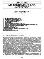
Fig. 7.15 with
an
expanded strain axis, which
is

necessary
for the
determination
of the
yield
strength.
The
nominal (approximate) stress
or the
strength
S
which
is
calculated
by
means
of Eq.
(7.8)
is
plotted
as the
ordinate.
The
abscissa
of the
engineering stress-strain plot
is the
nominal
strain,
which

is
defined
as the
unit elongation obtained when
the
change
in
length
is
divided
by the
original length
and has the
units
of
inch
per
inch
and is
designated
as n.
Thus,
for
ten-
sion,
n
=
^
=
^=^

(7.10)
€ €o
where
€ =
gauge length
and the
subscripts
O and /
designate
the
original
and
final
state, respectively. This equation
is
valid
for
deformation strains that
do not
exceed
the
strain
at the
maximum load
of a
tensile specimen.
It
is
customary
to

plot
the
data obtained
from
a
tensile test
as a
stress-strain curve
such
as
that illustrated
in
Fig. 7.16,
but
without including
the
word nominal.
The
reader then considers such
a
curve
as an
actual stress-strain curve, which
it
obviously
is
not.
The
curve plotted
in

Fig. 7.16
is in
reality
a
load-deformation curve.
If the
ordi-
nate axis were labeled load
(Ib)
rather than stress (psi),
the
distinction between
TABLE
7.3
Tensile
Test
Data
Material:
A40
titanium; condition: annealed; specimen
size:
0.505-in
diameter
by
2-in gauge
length;
A
0
=
0.200

in
2
Yield load
9 040
Ib
Maximum
load
14
950
Ib
Fracture
load
1 1
500
Ib
Final length
2.480
in
Final
diameter
0.352
in
Yield strength 45.2 kpsi
Tensile strength 74.75 kpsi
Fracture
strength 57.5 kpsi
Elongation
24%
Reduction
of

area
51.15%
Load,
Ib
1000
2000
3000
4000
5000
Gauge length,
in
2.0006
2.0012
2.0018
2.0024
2.0035
Load,
Ib
6000
7000
8000
9000
10000
Gauge length,
in
2.0044
2.0057
2.0070
2.0094
2.0140

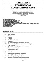
FIGURE
7.14
A
standard tensile specimen
of A40
titanium
at
various stages
of
loading,
(a)
Unloaded,
L
=
OIM
0
=
0.505
in,
€
0
=
2.000
in,
A
0
=
0.200
in
2

;
(b)
yield load
L
y
=
9040
Ib,
d
y
=
0.504
in,
Iy
=
2.009
in,
A
y
=
0.1995
in
2
;
(c)
maximum load
L
u
= 14 950
Ib,

d
u
=
0.470
in,
€
M
=
2.310
in,
A
u
=
0.173
in
2
;
(d)
fracture
load
L
7
=
11 500
Ib,
d
f
=
0.352
in,

€/=
2.480
in,
A
f
=
0.097
in
2
,
d
u
=
0.470
in.
NOMINAL STRAIN
n,in/in
FIGURE
7.15
The
elastic-plastic portion
of the
engineering stress-strain
curve
for
annealed
A40
titanium.
NOMINAL
(ENGINEERING)

STRESS,
kpsi
NOMINAL
STRAIN
n
FIGURE
7.16
The
engineering stress-strain
curve.
P =
proportional
limit,
Q =
elastic
limit,
Y=
yield
load,
U=
ultimate
(maximum)
load,
and
F
-
fracture
load.
strength
and

stress would
be
easier
to
make. Although
the
fracture load
is
lower than
the
ultimate load,
the
stress
in the
material just prior
to
fracture
is
much greater than
the
stress
at the
time
the
ultimate load
is on the
specimen.
7.9.2
True
Stress-Strain

The
tensile test
is
also used
to
obtain true stress-strain
or
true
stress-natural
strain
data
to
define
the
plastic stress-strain characteristics
of a
material.
In
this case
it is
necessary
to
record simultaneously
the
cross-sectional area
of the
specimen
and the
load
on it. For

round sections
it is
sufficient
to
measure
the
diameter
for
each load
recorded.
The
load-deformation data
in the
plastic region
of the
tensile test
of an
annealed titanium
are
listed
in
Table 7.4. These data
are a
continuation
of the
tensile
test
in
which
the

elastic data
are
given
in
Table 7.3.
The
load-diameter data
in
Table
7.4 are
recorded during
the
test
and the
remain-
der of the
table
is
completed
afterwards.
The
values
of
stress
are
calculated
by
means
of
Eq.

(7.9).
The
strain
in
this case
is the
natural strain
or
logarithmic
strain,
which
is
the sum of all the
infinitesimal nominal strains, that
is,
£
_Al
lf
Al
2
f
M
3
f
€o
€o
+
A€i
€o
+

A€i
+
A€
2
=
ln-^
(7.11)
<-o
The
volume
of
material remains constant during plastic deformation. That
is,
V
0
=
V
f
or
AaC
0
=
Af^
TABLE
7.4
Tensile Test
Datat
Load,
Ib
Diameter,

in
Area,
in
2
Area ratio Stress,
kpsi
Strain,
in/in
12000 0.501 0.197 1.015 60.9 0.0149
14000 0.493 0.191 1.048 73.5 0.0473
14500
0.486
0.186 1.075 78.0 0.0724
14950
0.470
0.173 1.155 86.5 0.144
14500 0.442 0.153 1.308 94.8 0.268
14000 0.425 0.142 1.410 99.4 0.344
11500
0.352 0.097 2.06 119.0 0.729
fThis
table
is a
continuation
of
Table
7-3.
Thus,
for
tensile

deformation,
Eq.
(7.11)
can be
expressed
as
E
=
In^
(7-12)
A
f
Quite
frequently,
in
calculating
the
strength
or the
ductility
of a
cold-worked
material,
it is
necessary
to
determine
the
value
of the

strain
£
that
is
equivalent
to the
amount
of the
cold work.
The
amount
of
cold
work
is
defined
as the
percent reduc-
tion
of
cross-sectional area
(or
simply
the
percent reduction
of
area) that
is
given
the

material
by a
plastic-deformation process.
It is
designated
by the
symbol
W and is
determined
from
the
expression
w
=
A
0
-A
f
(10Q)
(?
B)
AQ
where
the
subscripts
O
and/refer
to the
original
and the

final
area, respectively.
By
solving
for the
AJA
f
ratio
and
substituting
into
Eq.
(7.12),
the
appropriate
relation-
ship
between strain
and
cold work
is
found
to be
.,
lUU
/—
^
A
\
*"

=ln
m^w
(7
'
14)
The
stress-strain data
of
Table
7.4 are
plotted
in
Fig. 7.17
on
cartesian coordi-
nates.
The
most
significant
difference
between
the
shape
of
this stress-strain curve
and
that
of the
load-deformation curve
in

Fig.
7.16
is the
fact
that
the
stress contin-
ues to
rise until
fracture
occurs
and
does
not
reach
a
maximum value
as the
load-
deformation
curve does.
As can be
seen
in
Table
7.4 and
Fig. 7.17,
the
stress
at the

time
of the
maximum load
is 86
kpsi,
and it
increases
to 119
kpsi
at the
instant that
fracture
occurs.
A
smooth curve
can be
drawn through
the
experimental data,
but it
is
not a
straight line,
and
consequently many experimental points
are
necessary
to
accurately
determine

the
shape
and
position
of the
curve.
The
stress-strain data obtained
from
the
tensile test
of the
annealed
A40
titanium
listed
in
Tables
7.3 and 7.4 are
plotted
on
logarithmic coordinates
in
Fig. 7.18.
The
elastic portion
of the
stress-strain curve
is
also

a
straight line
on
logarithmic coordi-
nates
as it is on
cartesian coordinates. When plotted
on
cartesian coordinates,
the
slope
of the
elastic modulus
is
different
for the
different
materials. However, when
STRAIN
e,in/in
FIGURE
7.17 Stress-strain curve
for
annealed
A40
titanium.
The
strain
is
the

natural
or
logarithmic strain
and the
data
of
Tables
7.3 and 7.4 are
plot-
ted
on
cartesian coordinates.
plotted
on
logarithmic coordinates,
the
slope
of the
elastic modulus
is 1
(unity)
for
all
materials—it
is
only
the
height,
or
position,

of the
line that
is
different
for
differ-
ent
materials.
In
other
words,
the
elastic moduli
for all the
materials
are
parallel lines
making
an
angle
of 45°
with
the
ordinate
axis.
The
experimental
points
in
Fig:

7.18
for
strains greater than 0.01
(1
percent
plas-
tic
deformation) also
fall
on a
straight line having
a
slope
of
0.14.
The
slope
of the
stress-strain curve
in
logarithmic coordinates
is
called
the
strain-strengthening
expo-
nent
because
it
indicates

the
increase
in
strength that results
from
plastic strain.
It is
sometimes referred
to as the
strain-hardening
exponent,
which
is
somewhat mislead-
ing
because
the
real strain-hardening exponent
is the
Meyer exponent
p,
discussed
previously
under
the
subject
of
strain hardening.
The
strain-strengthening exponent

is
represented
by the
symbol
m.
The
equation
for the
plastic stress-strain line
is
a
=
a
0
£
m
(7.15)
and
is
known
as the
strain-strengthening
equation because
it is
directly related
to the
yield
strength.
The
proportionality constant

(T
0
is
called
the
strength
coefficient.
The
strength
coefficient
G
0
is
related
to the
plastic behavior
of a
material
in
exactly
FIGURE
7.18 Stress-strain
curve
for
annealed
A40
titanium
plotted
on
logarithmic

coordinates.
The
data
are the
same
as in
Fig. 7.17.
the
same manner
in
which
Young's modulus
E is
related
to
elastic behavior. Young's
modulus
E is the
value
of
stress associated
with
an
elastic strain
of
unity;
the
strength
coefficient
O

0
is the
value
of
stress associated
with
a
plastic strain
of
unity.
The
amount
of
cold work necessary
to
give
a
strain
of
unity
is
determined
from
Eq.
(7.14)
to be
63.3 percent.
For
most materials there
is an

elastic-plastic region between
the two
straight lines
of
the
fully
elastic
and
fully
plastic portions
of the
stress-strain curve.
A
material that
has
no
elastic-plastic region
may be
considered
an
"ideal"
material because
the
study
and
analysis
of its
tensile properties
are
simpler. Such

a
material
has a
com-
plete stress-strain relationship that
can be
characterized
by two
intersecting straight
lines,
one for the
elastic region
and one for the
plastic region. Such
a
material would
have
a
stress-strain curve similar
to the one
labeled
/in
Fig. 7.19.
A few
real materi-
als
have
a
stress-strain curve that approximates
the

"ideal"
curve. However, most
engineering materials have
a
stress-strain curve that resembles curve
O in
Fig. 7.19.
These materials appear
to
"overyield";
that
is,
they have
a
higher yield strength than
the
"ideal"
value,
followed
by a
region
of low or no
strain strengthening before
the
fully
plastic region begins. Among
the
materials that have this type
of
curve

are
steel,
stainless steel, copper, brass alloys, nickel alloys,
and
cobalt alloys.
Only
a few
materials have
a
stress-strain curve similar
to
that labeled
U in
Fig.
7.19.
The
characteristic feature
of
this type
of
material
is
that
it
appears
to
"under-
yield";
that
is, it has a

yield strength that
is
lower than
the
"ideal"
value. Some
of the
fully
annealed aluminum alloys have this type
of
curve.
7.70
TENSILEPROPERTIES
Tensile
properties
are
those mechanical properties obtained
from
the
tension test;
they
are
used
as the
basis
of
mechanical design
of
structural components more fre-
quently than

any
other
of the
mechanical
properties.
More tensile data
are
available
for
materials than
any
other type
of
material property data. Frequently
the
design
engineer must base
his or her
calculations
on the
tensile properties even under
FIGURE
7.19 Schematic representation
of
three types
of
stress-
strain
curves.
/ is an

"ideal" curve,
and O and U are two
types
of
real
curve.
cyclic,
shear,
or
impact loading simply because
the
more appropriate mechanical
property data
are not
available
for the
material
he or she may be
considering
for a
specific
part.
All the
tensile
properties
are
defined
in
this
section

and are
briefly dis-
cussed
on the
basis
of the
tensile test described
in the
preceding section.
7.10.1
Modulus
of
Elasticity
The
modulus
of
elasticity,
or
Young's
modulus,
is the
ratio
of
stress
to the
corre-
sponding strain during elastic deformation.
It is the
slope
of the

straight-line (elas-
tic) portion
of the
stress-strain curve when drawn
on
cartesian coordinates.
It is
also known,
as
indicated previously,
as
Young's modulus,
or the
proportionality
constant
in
Hooke's
law,
and is
commonly designated
as E
with units
of
pounds
per
square inch (pascals)
or the
equivalent.
The
modulus

of
elasticity
of the
titanium
alloy
whose tensile data
are
reported
in
Table
7.3 is
shown
in
Fig. 7.15, where
the
first
four
experimental data points
fall
on a
straight line having
a
slope
of
16.8 Mpsi.
7.10.2
Proportional Limit
The
proportional limit
is the

greatest stress which
a
material
is
capable
of
develop-
ing
without
any
deviation
from
a
linear proportionality
of
stress
to
strain.
It is the
point
where
a
straight line drawn through
the
experimental data points
in the
elas-
tic
region
first

departs
from
the
actual stress-strain curve. Point
P in
Fig. 7.16
is the
proportional limit
(20
kpsi)
for
this titanium alloy.
The
proportional limit
is
very sel-
dom
used
in
engineering specifications because
it
depends
so
much
on the
sensitiv-
ity
and
accuracy
of the

testing equipment
and the
person plotting
the
data.
7.10.3
Elastic
Limit
The
elastic
limit
is the
greatest stress which
a
material
is
capable
of
withstanding
without
any
permanent deformation
after
removal
of the
load.
It is
designated
as
point

Q in
Fig. 7.16.
The
elastic limit
is
also very seldom used
in
engineering
specifi-
cations because
of the
complex testing procedure
of
many successive loadings
and
unloadings
that
is
necessary
for its
determination.
7.10.4
Yield Strength
The
yield strength
is the
nominal stress
at
which
a

material undergoes
a
specified
permanent deformation.
There
are
several methods
to
determine
the
yield strength,
but the
most reliable
and
consistent method
is
called
the
offset
method. This
approach requires that
the
nominal stress-strain diagram
be
first
drawn
on
cartesian
coordinates.
A

point
z is
placed along
the
strain axis
at a
specified distance
from
the
origin,
as
shown
in
Figs. 7.15
and
7.16.
A
line parallel
to the
elastic modulus
is
drawn
from
Z
until
it
intersects
the
nominal stress-strain curve.
The

value
of
stress corre-
sponding
to
this intersection
is
called
the
yield strength
by the
offset
method.
The
dis-
tance
OZ is
called
the
offset
and is
expressed
as
percent.
The
most common
offset
is
0.2
percent, which corresponds

to a
nominal strain
of
0.002 in/in. This
is the
value
of
offset
used
in
Fig. 7.15
to
determine
the
yield strength
of the A40
titanium.
An
offset
of
0.01 percent
is
sometimes used,
and the
corresponding nominal stress
is
called
the
proof
strength,

which
is a
value very close
to the
proportional limit.
For
some nonferrous materials
an
offset
of 0.5
percent
is
used
to
determine
the
yield
strength.
Inasmuch
as all
methods
of
determining
the
yield strength give somewhat
differ-
ent
values
for the
same material,

it is
important
to
specify
what method,
or
what
off-
set,
was
used
in
conducting
the
test.
7.10.5
Tensile
Strength
The
tensile
strength
is the
value
of
nominal stress obtained when
the
maximum
(or
ultimate)
load that

the
tensile specimen supports
is
divided
by the
original cross-
sectional area
of the
specimen.
It is
shown
as
S
u
in
Fig. 7.16
and is
sometimes called
the
ultimate strength.
The
tensile strength
is a
commonly used property
in
engineer-
ing
calculations even though
the
yield strength

is a
measure
of
when plastic defor-
mation
begins
for a
given material.
The
real
significance
of the
tensile strength
as a
material property
is
that
it
indicates what maximum load
a
given part
can
carry
in
uniaxial
tension without breaking.
It
determines
the
absolute maximum limit

of
load
that
a
part
can
support.
7.10.6
Fracture
Strength
The
fracture
strength,
or
breaking
strength,
is the
value
of
nominal stress
obtained
when
the
load carried
by a
tensile specimen
at the
time
of
fracture

is
divided
by its
original
cross-sectional
area.
The
breaking strength
is not
used
as a
material prop-
erty
in
mechanical design.
7.10.7
Reduction
of
Area
The
reduction
of
area
is the
maximum change
in
area
of a
tensile specimen divided
by

the
original area
and is
usually expressed
as a
percent.
It is
designated
as
A
1
.
and
is
calculated
as
follows:
Ar
=
A
°~
Af
(1OQ)
(7.16)
AQ
where
the
subscripts
O
and/refer

to the
original area
and
area
after
fracture,
respec-
tively.
The
percent reduction
of
area
and the
strain
at
ultimate load
e
M
are the
best
measure
of the
ductility
of a
material.
7.10.8
Fracture
Strain
The
fracture

strain
is the
true strain
at
fracture
of the
tensile specimen.
It is
repre-
sented
by the
symbol
e/
and is
calculated
from
the
definition
of
strain
as
given
in Eq.
(7.12).
If the
percent reduction
of
area
A
r

is
known
for a
material,
the
fracture strain
can
be
calculated
from
the
expression
^
ln
w=z
^
7.10.9
Percentage
Elongation
The
percentage elongation
is a
crude measure
of the
ductility
of a
material
and is
obtained when
the

change
in
gauge length
of a
fractured tensile specimen
is
divided
by
the
original gauge length
and
expressed
as
percent.
Because
of the
ductility
rela-
tionship,
we
express
it
here
as
D
c
=
itzA(100)
(7.18)
Since

most materials exhibit nonuniform deformation before fracture occurs
on a
tensile
test,
the
percentage elongation
is
some kind
of an
average value
and as
such
cannot
be
used
in
meaningful
engineering calculations.
The
percentage elongation
is not
really
a
material propety,
but
rather
it is a
com-
bination
of a

material property
and a
test condition.
A
true material property
is not
significantly
affected
by the
size
of the
specimen. Thus
a
^-in-diameter
and a
H-in-
diameter
tensile specimen
of the
same material give
the
same values
for
yield
strength, tensile strength, reduction
of
area
or
fracture strain, modulus
of

elasticity,
strain-strengthening
exponent,
and
strength coefficient,
but a
1-in gauge-length
specimen
and a
2-in gauge-length specimen
of the
same material
do not
give
the
same
percentage elongation.
In
fact,
the
percentage elongation
for a
1-in gauge-
length
specimen
may
actually
be 100
percent greater than that
for the

2-in gauge-
length
specimen even when they
are of the
same diameter.
7.77
STRENGTH, STRESS,
AND
STRAIN RELATIONS
The
following relationships between strength, stress,
and
strain
are
very
helpful
to a
complete understanding
of
tensile
properties
and
also
to an
understanding
of
their
use in
specifying
the

optimum material
for a
structural part. These relationships also
help
in
solving
manufacturing
problems where
difficulty
is
encountered
in the
fabri-
cation
of a
given part because they enable
one to
have
a
better concept
of
what
can
be
expected
of a
material during
a
manufacturing process.
A

further
advantage
of
these relations
is
that they enable
an
engineer
to
more readily determine
the
mechanical
properties
of a
fabricated part
on the
basis
of the
original properties
of
the
material
and the
mechanisms involved with
the
particular process used.
7.11.1
Natural
and
Nominal Strain

The
relationship between these
two
strains
is
determined
from
their definitions.
The
expression
for the
natural strain
is e =
In
(€//€0).
The
expression
for the
nominal
strain
can be
rewritten
as
€//€
0
= n
+
!.When
the
latter

is
substituted into
the
former,
the
relationship between
the two
strains
can be
expressed
in the two
forms
£
=
In
(n
+ 1) exp (e) = n + 1
(7.19)
7.11.2
True
and
Nominal
Stress
The
definition
of
true stress
is a =
LIAi.
From constancy

of
volume
it is
found
that
A/
=
A
0
(V^
1
-),
so
that
L
/€,-\
a=
^fej
which
is the
same
as
O
=
If
1
+
J)
(7.20)
[S

exp (e)
7.11.3
Strain-Strengthening Exponent
and
Maximum-Load Strain
One of the
more
useful
of the
strength-stress-strain relationships
is the one
between
the
strain-strengthening exponent
and the
strain
at
maximum load.
It is
also
the
sim-
plest, since
the two are
numerically equal, that
is, m =
z
u
.
This relation

is
derived
on
the
basis
of the
load-deformation curve shown
in
Fig. 7.20.
The
load
at any
point
along this curve
is
equal
to the
product
of the
true stress
on the
specimen
and the
corresponding
area.
Thus
L =
oA
DEFORMATION
AREA

FIGURE
7.20
A
typical load-deformation curve showing unload-
ing
and
reloading
cycles.
Now,
since
o
-
o
0
8
m
and
1
A
0
A
AQ
8 =
In
—*-
or A
=
7—
A exp
(e)

the
load-strain relationship
can be
written
as
L =
OoA
0
8
m
exp
(-e)
The
load-deformation curve shown
in
Fig. 7.20
has a
maximum,
or
zero-slope,
point
on it.
Differentiating
the
last equation
and
equating
the
result
to

zero gives
the
simple expression
8 = m.
Since this
is the
strain
at the
ultimate load,
the
expression
can be
written
as
8
M
=
m
(7.21)
7.11.4
Yield
Strength
and
Percent
Cold
Work
The
stress-strain characteristics
of a
material obtained

from
a
tensile test
are
shown
in
Fig. 7.18.
In the
region
of
plastic deformation,
the
relationship between stress
and
strain
for
most materials
can be
approximated
by the
equation
a =
o
0
8
w
.
When
a
load

is
applied
to a
tensile specimen that causes
a
given amount
of
cold
work
W
(which
is
a
plastic strain
of
e
w
),
the
stress
on the
specimen
at the
time
is
a
w
and is
defined
as

ov
=
a
0
(ew)
w
(7.22)
Of
course,
o>
is
also equal
to the
applied load
L
w
divided
by the
actual cross-
sectional area
of the
specimen
A
w
.
If
the
preceding tensile specimen were immediately unloaded
after
reading

L
w
,
the
cross-sectional area would increase
to
AW
from
A
w
because
of the
elastic recov-
ery
or
springback that occurs when
the
load
is
removed. This elastic recovery
is
insignificant
for
engineering calculations with regard
to the
strength
or
stresses
on
a

part.
If
the
tensile specimen that
has
been stretched
to a
cross-sectional area
of
A'
w
is
now
reloaded,
it
will
deform elastically until
the
load
L
w
is
approached.
As the
load
is
increased above
L
w
,

the
specimen
will
again deform plastically. This unloading-
reloading
cycle
is
shown graphically
in
Fig. 7.20.
The
yield load
for
this previously
cold-worked
specimen before
the
reloading
is
A
w
.
Therefore,
the
yield strength
of
the
previously cold-worked (stretched) specimen
is
approximately

(s,V=^
A
w
But
since
A
W
=
A
W
,
then
s<?
\
-
LW
(Jy)w r-
^
1
W
By
comparing
the
preceding equations,
it is
apparent that
(Sy)w
— GW
And by
substituting this last relationship into

Eq.
(7.22),
we get
(Sy)
w
=
G
0
(e
w
)
m
(7.23)
Thus
it is
apparent that
the
plastic portion
of
the
a - e
curve
is
approximately
the
locus
of
yield strengths
for a
material

as a
function
of the
amount
of
cold
work. This rela-
tionship
is
valid only
for the
axial tensile yield strength
after
tensile deformation
or
for
the
axial compressive yield strength
after
axial deformation.
7.11.5
Tensile
Strength
and
Cold
Work
It is
believed
by
materials

and
mechanical-design engineers that
the
only relation-
ships between
the
tensile strength
of a
cold-worked material
and the
amount
of
cold
work
given
it are the
experimentally determined tables
and
graphs that
are
provided
by
the
material manufacturers
and
that
the
results
are
different

for
each
family
of
materials. However,
on the
basis
of the
concepts
of the
tensile test presented here,
two
relations
are
derived
in
Ref. [7.1] between tensile strength
and
percent cold
work
that
are
valid when
the
prior cold work
is
tensile. These relations
are
derived
on the

basis
of the
load-deformation characteristics
of a
material
as
represented
in
Fig. 7.20. This model
is
valid
for all
metals that
do not
strain age.
Here
we
designate
the
tensile strength
of a
cold-worked
material
as
(S
u
)
w
,
and we

are
interested
in
obtaining
the
relationship
to the
percent cold work
W. For any
specimen that
is
given
a
tensile deformation such that
A
w
is
equal
to or
less than
A
u
,
we
have,
by
definition, that
/c\
_
LU

(?u)w
77
A
w
And
also,
by
definition,
L
u
=
A
0
(Sw)
0
where
(S
u
)
0
=
tensile strength
of the
original non-cold-worked specimen
and
A
0
= its
original area.
The

percent cold work associated with
the
deformation
of the
specimen
from
A
0
toA
w
is
w=
A
0
-A
W(m
^
or
w
=
AQ^
AQ AQ
where
w
=
W/100.
Thus
Aw =
Ao(I-W)
By

substitution into
the
first
equation,
^=4SrS
^
Of
course, this expression
can
also
be
expressed
in the
form
(S
M
V=
(S
M
)o
exp(e)
(7.25)
Thus
the
tensile
strength
of
a
material
that

is
p
restrained
in
tension
to a
strain
less
than
its
ultimate
load
strain
is
equal
to its
original
tensile
strength
divided
by one
minus
the
fraction
of
cold
work.
This relationship
is
valid

for
deformations less than
the
defor-
mation associated with
the
ultimate load. That
is, for
A
w
<
A
u
or
e
w
^
£
M
Another relationship
can be
derived
for the
tensile strength
of a
material that
has
been previously cold-worked
in
tension

by an
amount greater than
the
deformation
associated with
the
ultimate load. This analysis
is
again made
on the
basis
of
Fig.
7.20.
Consider another standard tensile specimen
of
1020 steel that
is
loaded beyond
L
u
(12 000
Ib)
to
some load
L
z
,
say,
10 000

Ib.
If
dead weights were placed
on the end
of
the
specimen,
it
would break catastrophically when
the 12
000-lb
load
was
applied.
But if the
load
had
been applied
by
means
of a
mechanical screw
or a
hydraulic
pump, then
the
load would drop
off
slowly
as the

specimen
is
stretched.
For
this particular example
the
load
is
considered
to be
removed instantly when
it
drops
to
L
z
or 10 000
Ib.
The
unloaded specimen
is not
broken, although
it may
have
a
"necked"
region,
and it has a
minimum cross-sectional area
A

z
=
0.100
in
2
and a
diameter
of
0.358
in. Now
when this same specimen
is
again loaded
in
tension,
it
deforms
elastically until
the
load reaches
L
z
(10 000
Ib)
and
then
it
deforms plasti-
cally.
But

L
z
is
also
the
maximum value
of
load that this specimen reaches
on
reload-
ing.
It
never again
will
support
a
load
of
L
u
= 12 000
Ib.
On
this basis,
the
yield
strength
of
this specimen
is

/c
,
L
z
IQQQO
nnonn
.
(
^
=
^=-oior
=99200psl
And the
tensile strength
of
this previously
deformed
specimen
is
^-t-S-*™*
7.11.6
Ratio
of
Tensile
Strength
to
Brinell
Hardness
It is
commonly known

by
mechanical-design engineers that
the
tensile strength
of a
steel
can be
estimated
by
multiplying
its
Brinell hardness number
by
500.
As
stated
earlier, this
fact
led to the
wide acceptance
of the
Brinell hardness scale. However,
this ratio
is not 500 for all
materials—it
varies
from
as low as 450 to as
high
as

1000
for
the
commonly used metals.
The
ratio
of the
tensile strength
of a
material
to its
Brinell hardness number
is
identified
by the
symbol
K
B
,
and it is a
function
of
both
the
load used
to
determine
the
hardness
and the

strain-strengthening exponent
of
the
material.
Since
the
Brinell hardness number
of a
given material
is not a
constant
but
varies
in
proportion
to the
applied load,
it
then
follows
that
the
proportionality
coefficient
KB
is not a
constant
for a
given material,
but it too

varies
in
proportion
to the
load
used
in
determining
the
hardness.
For
example,
a 50
percent cobalt alloy (L605
or
HS25)
has a
Brinell hardness number
of 201
when tested with
a
3000-kg load
and a
hardness
of
only
150
when
tested
with

a
500-kg load. Since
the
tensile strength
is
about
145 000 psi for
this annealed alloy,
the
value
for
K
B
is
about
970 for the low
load
and
about
730 for the
high
load.
Since
the
material
is
subjected
to
considerable plastic deformation when both
the

tensile strength
and the
Brinell hardness
are
measured, these
two
values
are
influ-
enced
by the
strain-strengthening exponent
m for the
material. Therefore,
K
B
must
also
be a
function
of m.
Figure 7.21
is a
plot
of
experimental data obtained
by
this author over
a
number

of
years that shows
the
relationships between
the
ratio
K
B
and the two
variables
strain-strengthening exponent
m and
diameter
of the
indentation, which
is a
func-
tion
of the
applied
load.
From
these
curves
it is
apparent
that
K
8
varies directly with

m and
inversely
with
the
load
or
diameter
of the
indentation
d. The
following
exam-
ples
will
illustrate
the
applicability
of
these curves.
A
test
was
conducted
on a
heat
of
alpha brass
to see how
accurately
the

tensile
strength
of a
material could
be
predicted
from
a
hardness test when
the
strain-
strengthening exponent
of the
material
is not
known.
Loads
varying
from
200 to
2000
kg
were applied
to a
10-mm
ball, with
the
following
results:
Load,

kg 200 500
1000 1500 2000
Diameter,
mm
2.53 3.65 4.82 5.68 6.30
FIGURE
7.21 Relationships between
the
SJH
B
ratio
(K
B
)
and the
strain-strengthening
exponent
m. D
=
diameter
of the
ball,
and d -
diameter
of the
indentation. Data
are
based
on
experimental results

obtained
by the
author.
When plotted
on
log-log paper,
these
data
fall
on a
straight line having
a
slope
of
2.53, which
is the
Meyer strain-hardening exponent
n. The
equation
for
this straight
line
is
L
-18.8d
253
Since,
for
some metals,
m =

n-2,
the
value
of m is
0.53.
For
ease
in
interpreting Fig. 7.21,
the
load corresponding
to an
indentation
of 3
mm
is
calculated
from
Eq.
(7.2)
as 43.
K
B
can now be
determined
from
Fig. 7.21
as
890.
Thus

the
tensile strength
is
S
u
=
K
8
H
8
=
890(43)
= 38 300
psi.
In a
similar
fash-
ion,
the
load
for a
5-mm diameter
is 110 kg, and the
corresponding Brinell hardness
number
is 53.
From Fig. 7.21,
the
value
of

K
8
is
found
to be
780,
and the
tensile
strength
is
estimated
as
S
n
=
K
8
H
8
=
780(53)
= 41 300
psi.
The
average value
of
these
two
calculated tensile strengths
is 39 800

psi.
The
experimentally determined value
of
the
tensile strength
for
this brass
was 40 500
psi, which
is
just
2
percent lower than
the
predicted value.
As
another example, consider
the
estimation
of
tensile strength
for a
material
when
its
typical strain-strengthening exponent
is
known. Annealed 3003 aluminum
has

an
average
m
value
of
0.28. What
is the
tensile strength
of a
heat
that
has a
Brinell hardness number
of 28
when measured with
a
500-kg load?
The
diameter
of
the
indentation
for
this hardness number
is
4.65. Then
from
Fig. 7.21
the
value

of
K
8
is
determined
as
535.
The
tensile strength
can
then
be
calculated
as
S
u
=
K
8
H
8
=
535(28)
= 15 000
psi.
7.72
IMPACTSTRENGTH
In
some cases
a

structural part
is
subject
to a
single, large, suddenly applied load.
A
standard
test
has
been
devised
to
evaluate
the
ability
of a
material
to
absorb
the
impact
energy through plastic deformation.
The
test
can be
described
as a
techno-
logical
one, like

the
Rockwell hardness test, rather than
as a
scientific
one.
The
val-
ues
obtained
by the
impact test
are
relative rather than absolute. They serve
as a
basis
of
comparison
and
specification
of the
toughness
of a
material.
The
impact strength
is the
energy, expressed
in
footpounds, required
to

fracture
a
standard
specimen with
a
single-impact blow.
The
impact strength
of a
material
is
frequently
referred
to as
being
a
measure
of the
toughness
of the
material, that
is, its
ability
to
absorb energy.
The
area under
the
tensile
stress-strain

curve
is
also
a
mea-
sure
of the
ability
of a
material
to
absorb energy (its toughness). Unfortunately,
there
is
only
a
very general relationship between these
two
different
measures
of
toughness;
namely,
if the
material
has a
large area under
its
tensile
stress-strain

curve,
it
also
has a
relatively high impact strength.
Most
imp
act-strength
data
are
obtained with
the two
types
of
notched specimens
shown
in
Fig. 7.22. Figure
7.22«
illustrates
the
Charpy V-notch specimen
as
well
as
how
the
impact load
is
applied. Figure

7.22b
does
the
same
for the
Izod
V-notch
specimen,
and the
details
of the
notch
are
shown
in
Fig. 7.22c.
There
are
several mod-
ifications
of the
standard V-notch specimen.
One is
called
the
keyhole notch
and
another
the
U-notch.

Both have
a
1-mm
radius
at the
bottom rather than
the
0.25-
mm
radius
of the
V-notch.
There
is no
correlation between
the
various types
of
notch-bar
impact-strength values. However,
the
Charpy V-notch impact-strength
value
is
considerably greater than
the
Izod V-notch value, particularly
in the
high
toughness

range.
The
impact-testing machine consists
of a
special base mounted
on the
floor
to
support
the
specimen
and a
striking hammer that swings through
an arc of
about
32-
in
radius, much like
a
pendulum. When
the
hammer
is
"cocked"
(raised
to a
locked
elevation),
it has a
potential energy that varies between

25 and 250 ft •
Ib,
depending
on the
mass
of the
hammer
and the
height
to
which
it is
raised. When
the
hammer
is
released
and
allowed
to
strike
the
specimen,
a
dial registers
the
energy that
was
absorbed
by the

specimen.
The
standards
specify
that
the
striking velocity must
be in
the
range
of 10 to 20
ft/s because velocities outside this range have
an
effect
on the
impact
strength.
FIGURE 7.22 Impact tests
and
specimens,
(a)
Charpy
L = 55 mm; (b)
Izod
L
= 15 mm; (c)
details
of the
notch.
The

impact strengths
of
some materials, particularly steel, vary significantly with
the
testing temperature. Figure 7.23 shows this variation
for a
normalized
AISI1030
steel.
At the low
testing temperature
the
fracture
is of the
cleavage type, which
has a
bright,
faceted appearance.
At the
higher temperatures
the
fractures
are of the
shear
type, which
has a
fibrous
appearance.
The
transition temperature

is
that temperature
that results
in 50
percent cleavage fracture
and 50
percent shear
fracture,
or it may
be
defined
as the
temperature
at
which
the
impact strength shows
a
marked drop.
The
nil-ductility
temperature
is the
highest temperature
at
which
the
impact strength
starts
to

increase above
its
minimum value. These
two
temperatures
are
shown
in
Fig.
7.23.
TEMPERATURE,
0
F
FIGURE 7.23 Charpy
V-notch
impact strength
of
1030 steel versus temperature.
A =
nil-ductility tem-
perature;
B =
transition temperature.
7.73
CREEPSTRENGTH
A
part
may
fail
with

a
load that induced stresses
in it
that
lie
between
the
yield
strength
and the
tensile
strength
of the
material even
if the
load
is
steady
and
con-
stant rather than alternating
and
repeating
as in a
fatigue
failure. This type
of
con-
stant loading causes
the

part
to
elongate
or
creep.
The
failure point
may be
when
the
part stretches
to
some specified length,
or it may be
when
the
part completely
fractures.
The
creep
strength
of a
material
is the
value
of
nominal stress that
will
result
in a

specified
amount
of
elongation
at a
specific temperature
in a
given length
of
time.
It
is
also defined
as the
value
of
nominal stress that induces
a
specified creep
rate
at a
specific
temperature.
The
creep strength
is
sometimes called
the
creep
limit.

The
creep
rate
is the
slope
of the
strain-time creep curve
in the
steady-creep region,
referred
to as a
stage
2
creep.
It is
illustrated
in
Fig. 7.24.
Most creep
failures
occur
in
parts that
are
exposed
to
high temperatures rather
than room temperature.
The
stress necessary

to
cause creep
at
room temperature
is
considerably higher than
the
yield strength
of a
material.
In
fact,
it is
just slightly less
than
the
tensile strength
of a
material.
The
stress necessary
to
induce creep
at a
tem-
perature that
is
higher than
the
recrystallization temperature

of a
material, however,
is
very low.
FIGURE 7.24
Creep
data
plotted
on
semilog
coordinates,
(a) Low
stress
(slightly
above
S
y
)
or low
temperature
(well below recrystallization);
(b)
mod-
erate
stress
(midway
between
S
y
and

S
u
)
or
moderate
temperature
(at
recrys-
tallization);
(c)
high
stress
(slightly below
S
u
)
or
high
temperature
(well
above
recrystallization).
The
elastic
elongations
are
designated
as
Oa,
Ob, and Oc.

The
specimens used
for
creep testing
are
quite similar
to
round tensile specimens.
During
the
creep test
the
specimen
is
loaded with
a
dead weight that induces
the
required nominal stress applied throughout
the
entire test.
The
specimen
is
enclosed
in
a
small round tube-type
furnace
to

maintain
a
constant temperature throughout
the
test,
and the
gauge length
is
measured
after
various time intervals. Thus
the
three
variables
that
affect
the
creep rate
of the
specimen
are (1)
nominal stress,
(2)
tem-
perature,
and (3)
time.
Figure
7.24 illustrates
the

most common method
of
presenting creep-test data.
Three
different
curves
are
shown. Curve
(a) is
typical
of a
creep test conducted
at a
temperature well below
the
recrystallization temperature
of the
material (room
temperature
for
steel)
and at a
fairly
high stress level, slightly above
the
yield
strength.
Curve
(a) is
also typical

of a
creep test conducted
at a
temperature near
the
recrystallization
temperature
of a
material
but at a low
stress level. Curve
(c) is
typ-
ical
of
either
a
high stress level, such
as one
slightly below
S
u
,
at a low
temperature,
or
else
a low
stress level
at a

temperature
significantly
higher than
the
recrystalliza-
tion temperature
of the
material. Curve
(b)
illustrates
the
creep rate
at
some inter-
mediate combination
of
stress
and
temperature.
A
creep curve consists
of
four
separate parts,
as
illustrated
with
curve
(b) in
Fig.

7.24.
These
are
explained
as
follows:
1. An
initial elastic extension
from
the
origin
O to
point
Ob.
2. A
region
of
primary creep,
frequently
referred
to as
stage
1
creep.
The
extension
occurs
at a
decreasing rate
in

this portion
of the
creep
curve.
3. A
region
of
secondary creep,
frequently
called
stage
2
creep.
The
extension occurs
at
a
constant rate
in
this region. Most creep design
is
based
on
this portion
of the
creep curve, since
the
creep rate
is
constant

and the
total extension
for a
given
number
of
hours
of
service
can be
easily calculated.
4. A
region
of
tertiary creep
or
stage
3
creep.
The
extension occurs
at an
increasing
rate
in
this region until
the
material
fractures.
ELONGATION

Another practical
way of
presenting creep data
is
illustrated
in
Fig. 7.25, which
is
a
log-log plot
of
nominal stress versus
the
second-stage creep rate expressed
as
per-
cent
per
hour with
the
temperature
as a
parameter. Figure 7.26 illustrates still
another type
of
plot that
is
used
to
present creep data where both

the
stress
and
tem-
perature
are
drawn
on
cartesian coordinates.
The
mechanism
of
creep
is
very complex inasmuch
as it
involves
the
movements
of
vacancies
and
dislocations, strain hardening,
and
recrystallization,
as
well
as
grain-
boundary

movements.
At low
temperatures, creep
is
restricted
by the
pile-up
of
dis-
locations
at the
grain boundaries
and the
resulting strain hardening.
But at
higher
temperatures,
the
dislocations
can
climb
out of the
original slip plane
and
thus per-
mit
further
creep.
In
addition, recrystallization,

with
its
resulting lower strength, per-
mits creep
to
occur readily
at
high temperatures.
CREEP
RATE,
%/hr
(LOG
SCALE)
FIGURE 7.25 Second-stage
creep
rate
versus nominal
stress.
A, B,
and C are for
low, medium,
and
high temperatures, respectively.
TEMPERATURE,
0
F
FIGURE 7.26 Second-stage
creep
rate
versus tem-

perature
and
nominal
stress.
A,
1%/h
creep
rate;
B,
0.1
%/h
creep
rate;
C,
0.001
%/h
creep
rate.
NOMINAL
STRESS
(LOG
SCALE)
NOMINAL STRESS