Sổ tay tiêu chuẩn thiết kế máy P14 potx

CHAPTER
11
MINIMIZING
ENGINEERING
EFFORT
Charles
R.
Mischke,
Ph.D.,
P.E.
Professor
Emeritus
of
Mechanical
Engineering
Iowa
State
University
Ames,
Iowa
11.1
INTRODUCTION/11.2
11.2
REDUCING
THE
NUMBER
OF
EXPERIMENTS
/11.3
11.3
SIMILITUDE/11.7

11.4
OPTIMALITY/11.9
11.5
QUADRATURE/11.13
11.6
CHECKING/11.15
REFERENCES/11.21
NOMENCLATURE
a
Distance, range number, bilaterial tolerance
b
Width, range number
C
Constant
D
Helix diameter
dim
Dimensional
operator
E
Young's modulus
E
n
Error
using
n
applications
of
Simpson's rule
e

t
The
/th
exponent
/
Function
f®
The
/th
derivative
of
function
/
F
Fundamental dimension
of
force, fractional reduction
of
interval
of
uncertainty
g
Function
h
Function, ordinate spacing
/
Index
/
Second area moment, value
of

integral
I
1
Approximate value
of
integral using
i
applications
of
Simpson's rule
k
Spring rate
K
1
J
Exponent
of
fundamental
dimension
in row
/,
of
parameter
y
in
dimen-
sional matrix
L
Fundamental dimension
of

length
€
Span,
left
In
Natural logarithm
m
Mass, subscript
of
model
n
Number
TV
Number
of
experiments
to
establish
a
robust
functional
relationship
among
n
parameters, number
of
function
evaluations
N'
Number

of
experiments
to
establish
a
robust
functional
relationship
among
dimensionless parameters
N
a
Number
of
active turns
in a
spring
N
n
Number
of pi
terms
in a
complete
set
p
Number
of
points necessary
to

establish
a
robust functional relationship
between
two
parameters
P
Load
Q
Fundamental dimension
of
charge
r
Rank
of
dimensional matrix,
right
s
Scale
factor,
the
ratio
of
model over prototype dimension
T
Fundamental dimension
of
time
x
Location parameter

x*
Abscissa
of
extreme
of a
function
Xe,
x
r
Range numbers
on
left
and
right, respectively
y
Transverse beam deflection
A
Tolerable
error
9
Fundamental dimension
of
temperature
K
1
The
/th
pi
term
£

Location
in
Simpson's rule application interval where error term
is
exact
77.7
INTRODUCTION
The old
carpenter's admonition "Measure twice,
cut
once"
reminds
us
that sound
preparatory
effort
avoids later
grief
in
terms
of
redoing
or
scrapping prior work
effort.
In
technical undertakings, engineering
effort
is
required long before work

starts.
Not
only must
it be
done correctly,
but
since
it is an
overhead cost,
it is
impor-
tant
that
it be
accomplished
in a
cost-efficient
manner without compromising
the
quality
of the
result.
In
order
to
accomplish this routinely, engineers have developed
and
adopted strategies, manners
of
approach that

are
routinely
mindful
of
effective
use of
engineering resources.
One
such strategy
is the
mathematical model.
It
gives
us
quantitative insight into
domains
that
are new to us. It is
unfortunate that
the
name mathematical model
is
commonly
applied
to
this tool,
for
mathematics does
not
intrinsically contain

the
reality.
It has to be
carefully
built
in if the
model
is to
satisfactorily describe nature.
Attention
focus
for
thinking
and
communicative processes
is
rooted
in and
well
served
by
concepts
of
system, boundary,
and
surroundings
or
control region, control
surface,
and

surroundings.
There
are
also notions
of
cause,
effect,
and
extent
as
sys-
tems interact with their surroundings.
We
recognize heat
and
work
effects,
tractive
effects,
charge
effects,
chemical
effects,
and
ballistic
effects
related
to
nuclear phe-
nomena.

It is in
these
effects
(and their quantitative expression) that reality
is
mod-
eled.
It is
when these
effects
are
combined with
notions
of
accountability,
or
balances,
and
first
principles that reality
can be
incorporated into mathematical
models
([11.1],
Chaps.
6,7).
Deterministic, deductive mathematical models
are
usually created using
the

fol-
lowing
steps
([11.1],
p.
228):
1.
Isolate
a
finite
or
infinitesimal
system
or
control region.
2.
Identify
the
significant
influences
of the
surroundings,
or
changes within
the
iso-
lated
system
or
control region.

3.
Qualify
significant
influences
or
changes with mathematical models
of
effects.
4.
Relate
influences
to
system
or
control-region behavior
by
using
first
principles.
5.
Limit,
if
necessary,
as
AJC,
Ay,
Az,
Ar,
etc., approach zero.
6.

Solve
the
resulting equation(s)
for
variable(s)
of
interest. Assumptions
or
judg-
ments
may be
required
to
make
a
solution possible.
7.
Check your work (see Sec.
11.6).
Engineers recognize that variability
is
omnipresent
in
nature
and
that measured
quantities
are
knowable only
in

terms
of
estimates
of
means
and
variances, distribu-
tional
forms,
and
confidence limits. This variability
or
uncertainty must
be
consid-
ered when judging
the
worth
of the
model results.
77.2
REDUCINGTHENUMBEROF
EXPERIMENTS
In
describing
the
functional
relationship between variables
Jt
1

and
Jc
2
,
it
takes
a
num-
ber of
experiments (points)
to
establish
a
satisfactory approximation
to the
func-
tional relationship. Consider that number
of
experiments
to be p. At
this
point
we
are
concerned
not
with
the
method
of

establishing
the
working approximation
(least-square
curve
fits,
for
example)
but
with
the
amount
of
effort
associated with
gathering
the
data points used
to
establish
that
relationship.
If the
level
of
effort
in
time
and
expense

is
proportional
to the
number
of
points
p, we use the
magnitude
of
p
as our
index
to
cost.
The
relationship between
Jt
1
and
X
2
can be
displayed
as a
data
string
on a
sheet
of
graph paper

([11.1],
pp.
139-160).
How
many
experiments
are
necessary
to
describe
a
phenomenon involving
n
parameters
Jc
1
,
Jt
2
, ,
Jt,,?
During
the
experiments necessary
to
relate
Jc
1
to
Jt

2
,
all
other parameters were held constant.
The
role
of
Jt
3
is
then introduced
by
perform-
ing p
experiments
at
level
(jt
3
)
t
,
(jc
3
)
2
, ,
(KS)P.
This places
p

contours
on the
Jt
1
Jt
2
graph.
Up to
this point
there
have
been/?
2
experiments.The
introduction
of the
third
parameter increased
the
level
of
effort
exponentially.
Similarly,
the
fourth
parameter
requires
p
pages

of p
curves
of p
points each.
The
total number
of
experiments
TV
necessary
for n
parameters using
p
points
for
each curve
is,
therefore,
N
=
p
n
~
l
(11.1)
If
p = 6 and n - 5,
then
N -
6

5
x
=
1296
experiments.
If the
cost
of
experimental
determination
is
$100
or
$1000
per
point, then quantitative understanding
is
pro-
hibitively
expensive.
Is
there
any
alternative
to
this investment
of
time
and
effort?

We
are
indebted
to
Buckingham,
who
suggested clustering parameters
in
dimen-
sionless groups. Instead
of
finding
the
relationship among
Rx
19
X
2
, ,Xn)
= O
Buckingham
suggested
finding
the
relationship among
g(7li,7C
2
,
.
,7l

n
_
r
)
=
0
where
r is the
rank
of the
matrix
of
dimensions.
The
level
of
effort
N'
is now
given
by,
after
Eq.
(11.1),
N'=p
n
~
r
~
l

(11.2)
The
ratio
N'IN
is,
using Eqs.
(11.1)
and
(11.2),
N'
n
n
~
r
~
l
1
—-£-
fll
^
N~
p"-
1
~p
r
(
^
If
the
rank

of the
matrix
of
dimensions
is 2 and 10
points
are
necessary, then
N'
1 1
TV
~
10
2
" 100
and
the
level
of
effort
has
been reduced
by a
factor
of
100.
Pi
terms
are
multiplicative clusters

of
parameters, formed
by
exploiting
the
rule
of
dimensional homogeneity.
The set
of
fundamental dimensions consists
of the
irre-
ducible
set of
force
F,
length
L,
time
T,
temperature
6, and
charge
Q.
Mass
can be
used instead
of
force.

A
velocity
V has the
dimensions
of
length/time,
or
LIT,
and
such
quantities
are
called secondary
or
derived quantities.
We can say
that
the
dimensions
of V,
dim(V
r
),
are LIT or
L
1
T"
1
,
or,

more completely,
dim(F)
=
FL
1
T-
1
Q
0
Q
0
(11.4)
Care
has to be
taken
to
establish
a
complete
set of
dimensionless clusters,
or pi
terms.
A
complete
set
means that
the
pi-term
set is the

exact counterpart
of the
parameter
set.
The
first
step
is to
construct
a
matrix
of
dimensions
for the
parameter
set.
If the
parameters
are
X^x
2
,
,X
n
and the
fundamental dimensions involved
are
force
F
and

length
L,
then
the
matrix
of
dimensions
is
displayed
as
Xi
X
2

X
n
F
\
KU
K
n
•
-
•
Ki
n
L
K
2
i

K
22
. . .
K
2n
For
example,
for a
helical compression spring,
the
spring rate
k is
affected
by the
number
of
active turns
N
a
,
wire diameter
d,
torsional modulus
G, and
helix diameter
D.
The
dimensions
are
dim(A:)

=
F
1
L'
1
dim(G)
=
F
1
Zr
2
dim(N
a
)
=
F
0
L
0
dim(D)
=
F
0
L
1
dim(d)
=
F
0
L

1
The
matrix
of
dimensions
for the
spring consists
of the
display
of the
exponents
of
the
fundamental dimensions
in
each
of the
parameters:
k
N
a
d G D
FlOOlO
L-I
O
1-21
The
rank
of
this matrix

is the
order
of the
largest nonzero determinant that
can be
found
in the
matrix. Since
the
right-hand determinant
-2
1
=1
-°
=
1
^°
is
nonzero,
the
rank
r is 2.
There
may be
several
of
these depending
on the
sequenc-
ing

of
parameters across
the
top.
It is
important
for
completeness that
a
nonzero
determinant
be
placed
on the
right
in the
matrix
of
dimensions.
The
number
of
mul-
tiplicative dimensionless clusters
or pi
terms
N
n
is
given

by
N
n
= n-r
(11.5)
A pi
term
is
formed
by
writing
Ti;
=
A^W/
2
<f
3
G
64
D^
(11.6)
The
dimensional operator
is
applied
as
follows:
dim(7i;)
=
dim(k

ei
)dim(N
a
e
^dim(d
e
^dim(G
e4
)dim(D
e5
)
=
(F
l
L-
l
)\F
Q
L^(F
Q
L
l
^(F
l
L-
2
)^(F
Q
L
1

)^
For the
force dimension,
^O
_
peipOpOpe
4
pO
The
exponent
of F
must
be the
same
on
both sides:
O
=
(I)C
1
+
(G)C
2
+
(0)*
3
+
(Ve
4
+

(0)*
5
Note that
the
coefficients
of the
exponential equation agree with
the
first
row of the
dimensional matrix.
In
other words,
the
exponential equation associated with
any
fundamental
dimension
can be
written
by
inspection
from
the
matrix
of
dimensions.
The two
exponential equations
are

ei
+
e
4
= O
(for force dimension)
(11.7)
-ei
+
e
3
-2e
4
+
e
5
=
O
(for length dimension)
(11.8)
There
are two
exponential equations
(r is 2) and
five
exponents
(n is 5), and so
three
exponents
are

mathematically arbitrary.
We
will
choose them
so
that
the
first
three
parameters
k,
N
a
,
and d
each appear
in
only
one pi
term. Such parameters
are
used
to
control their
pi
terms independently,
if
necessary.
It
is

useful
to
display
a
matrix
of
solutions. There
are n - r = 5 - 2 = 3 pi
terms.
(/c)
(N
a
)
(d) (G) (D)
C
1
C
2
C
3
64
C
5
Tl
1
1 O O
Tl
2
O 1 O
Tl

3
O O 1
Solving
Eqs.
(11.7)
and
(11.8)
to
complete
the
matrix
of
solutions
is
done
as
follows:
e
4
=
-C
1
e
5
=
2e
4
+
e
l

-e
3
For
e\
=
I,e
2
=
O,^
3
=
O,
For
e\
-O,e^
=
1,^s
=
O,
For
ei
=
0,e
2
=
0,e
3
= l,
64=
-1

64
= 0
e
4
=0
e
5
= -2 + 1 = -1
e
5
= O
e
5
= -1
The
completed matrix
of
solutions
is
(*)
(AQ
(d) (G) (D)
ei
e
2
e
3
e
4
e

5
Tii
1
00-1-1
=>
K
1
=
^G-
1
D-
1
K
2
O 1 O O O =>
Ti
2
=
Ni
U
3
O O 1 O -1
=>n
3
=
d
l
D-
1
and

the pi
terms
can be
displayed
as
K
1
=
J^
K
2
=
JV
0
K
3
=
A
Recall that
if
p = 10,
then
the
number
of
experiments
from
Eq.
(11.1)
is N =

p
n
~
1
=
10
5
~
l
=
10,000.
By
using Buckingham's multiplicative
dimensionless
clusters,
Eq.
(11.2)
gives
AT
-
10
5
-
2
-
1
=
100.
Can we
reduce

the
hundred experiments even more?
If we can
introduce
infor-
mation
we
already
know,
we
can.
Two
identical springs
in
series
(end
to
end) have
twice
the
turns
and
half
the
spring rate;
in
other words,
TIiTi
2
=

Ci(TC
3
).
The
problem
reduces
to
finding
TTiTT
2
=
/Z(Tl
3
)
Now
there
are
only
10
experiments
to be
performed.
As an aid to
partitioning
our
thinking
so
that
we can
deal with

one
thing
at a
time,
we can use the
method
of
deriva-
tives.
Since there
are
three
pi
terms
in the
spring problem,
we
seek
the
function
Tl
1
=
/Zi(TC
2
,
TC
3
)
It

follows
then that
,
oKi
,
aTCi
j
/t
t
n\
(In
1
=—-
^TC
2
+-^-
dn
3
(11.9)
OTC
2
OK
3
In
noting
the
inverse proportionality between
KI
and
Ti

2
from
before,
we
write
Ci
3TCi
Ci
TCiTl
2
TCi
/r
• \
TCi
= —
^—
= -
—7
= -
—r~
= - —
(from
prior experience)
TC
2
3TC
2
TC
2
TC

2
TC
2
When
we
conduct
the p
experiments
and
find
UiIn
3
—
C
2
(TC
2
)
at
constant
TC
2
,
we
have
TC
1
=
C
2

TC
3
*
!^
=
4C
2
TC^
=
4
^nI
=
4
—
(from
test)
OK
3
TC
3
TC3
Thus
Eq.
(11.9)
becomes
,
TCi
6?TC
2
A

TCi
»
dTCi
= -
——-
+ 4
—-
dn
3
TC
2
TC
3
Dividing through
by
TC
1
renders
the
equation exact
and
integrable term
by
term:
dTCi
^Tc
2
A
dn
3

=
—
h
4
TCi
^2
7C3
In
TCi
- -
In
TC
2
+
In
TC
3 +
In
C
or
TC
1
-C^-
(11.10)
7C2
The
constant
C can be
found
from

the p
experiments. Equation
(11.10)
can be
writ-
ten as
d
4
G
SD
3
N
0
Do not
underestimate
the
power
of
Buckingham's suggestion
and the
incorporation
of
a
priori knowledge with test results
to
enormously reduce
the
effort.
77.3
SIMILITUDE

The
first
similitude equation
of
which
we
have
a
record dates
to the
fourth
century
B.C.,
when
it was
recorded
by
Philon
of
Byzantium
for the
ballista
[11.2].
It
related
what
we now
call
the
mass

of the
projectile
to be
thrown
to the
diameter
of the
tor-
sional springs used
as
^=(—T
am)'
di
\m
2
/
Ever since, engineers have embroidered
on
this idea with
useful
results.
In the
con-
text
of
Sec.
11.2,
this
is a
relationship between

two pi
terms.
The
idea that
will
be
use-
ful
to us can be
related
to the
helical spring example
of
Sec.
11.2.
With
a
spring
in
hand,
one can
quantitatively express
KI
=
klGD.
However, knowing that
KI
is 0.5 x
10~
5

will
not
identify
the
spring parameters. What constructing
the pi
term
has
done
is map all
springs with
Ti
1
= 0.5 x
10~
5
onto
a
single coordinate. This suggests
that
one
can
model
one
spring
with
K
1
= 0.5 x
10~

5
with
another that also
has
K
1
= 0.5 x
10~
5
,
but
is
of
differing
material, spring rate,
and
helix diameter. This
can be
useful
in
adjust-
ing
to
size
and
capacity constraints
on
test instrumentation.
For a
timber beam

of
cross section
b
wide
and d
deep, with
a
concentrated load
P
located
a
distance
a
from
the
left
support,
and a
span
of
€,
the
transverse deflection
y
at a
distance
x
from
the
left

support
is
described
by
fty,
a,
b,
d,
x,
P,
E,
€)
-
O
or
equally
as
well
by
Buckingham's
pi
terms
as
ly_a
b_d_±_P_\
0
*\ee
e
ee
EP)

Suppose
we
wish
to
model
the
timber beam
in a
different
size
and
material.
The
function
g in
model terms
is
written
(y
m
OSL
brn_
dm
£m
Pm
\
=
Q
I
f

'
f
'
f
'
f
'
f
'Ff
2
I
\^m
^m
^m ^m ^m
-^m^m
/
In
order
for
this
to be a
model, corresponding
pi
terms must
be
identical. Since
yjt
m
=
yW,

it
follows
that
y
m
=
^-y
=
sy
where
s is the
scale
factor,
s =
€
m
/€.
The
other linear dimensions
are
a
m
=
sa
b
m
=
sb
d
m

=
sd
x
m
= sx
The
sixth
pi
terms
are
equated,
from
which
p _
*£>m"m
_ 2
^m
p
Pm
~
E^
~
S
~E
P
The
load
P
m
is the

mandatory load
on the
model corresponding
to P. The
location
at
which
to
measure
the
transverse deflection
is
x
m
= sx. If a
steel model
is
1/10
size
and
the
prototype load
is
4800
lbf,
the
model load
P
m
is

f
In a
book
addressing
machine
design,
shouldn't
this
be Eq.
(1.1)?
^O
v
10
6
P
m
=
O.I
2
13X
1
Q
6
4800-960lbf
and
the
prototype deflection
is y =
yjs.
T

1.4
OPTIMALITY
The
subject
of
optimality
is
extensive
[11.3],
[11.4].
Our
purpose here
is to
examine
the
efficiency
of an
optimization process
itself,
for any
internal wasted
effort
in a
computer-coded algorithm
is
incessantly repeated.
A
unimodal
function
is one

that
monotonically increases, monotonically decreases,
or
monotonically increases then
decreases.
If the
original interval containing
a
maximum
has the
range numbers
JQ,
x
r
and
there
are n
ordinates equally spaced within
the
interval (but
no
ordinates
at
Xf
or
Jt
r
),
then
the

ordinate spacing
is
h
=
*
L
^
L
n
+
l
By
examining
the
ordinates,
the
final
interval
of
uncertainty
is
reduced
to
2h,
and the
fractional
reduction
in the
interval
of

uncertainty
is
F
_
2h
_2(x
r
-x<)/(n
+ l) _ 2
x
r
-Xf
x
r
-x
f
n + l
Solving
for n
gives,
for
fractional reduction
F and
bilateral
tolerance,
jc*
± a
locations
of
the

extreme, respectively:
"-[H-fe?l
(1L12)
When
n is not an
integer,
it is
rounded
up. For
F=
0.001,
KoM-
1
I=P
000
-
1
^
1999
Thus,
1999 function evaluations
are
required.
See
Ref.
[11.1],
pp.
278-290.
Instead
of

expending
all
ordinates simultaneously,
one can
spend
a
few, reduce
the
interval somewhat,
and
keep repeating
the
process.
For
equally spaced ordinates,
the
optimal procedure
([11.3],
p.
282)
is
spending
n as 3 + 2 + 2
+
-
••.
This
is
called
interval

halving.
The
total number
of
function
evaluations
N
spent this
way is
N=
\
l+
^L]
=
L
881n
JLZ*
J
(11
.13)
L
In
2
Jodd
+
L a
Jodd
+
v
'

For
F
-0.001,
„
F
1
+
IhL^OOOl
=[2
o.
93]odd
+
=
21
L
m
2
Jodd
+
This
is a
remarkable reduction
in
effort.
One can do
better
by
relaxing
the
equal

spacing
stipulation
and
spending
([11.1],
pp.
284-289)
ordinates
2
+1 +1
+ • • •.
Under
these circumstances,
for
fractional
and
bilateral tolerance reductions, respectively,
^['^nO^OB^l'h"^].
<
1U4
>
and
the
method
is
called golden section.
For
F=
0.001,
,,

L
In
0.001
1
ri
.
a
,
_
^^^ln
0.618033
989
J
+
=
[1535]+
=
16
which
is
approximately three-fourths
as
many
function
evaluations
as
were required
for
interval halving.
Can one do

better?
The
answer
is a
qualified
yes.
A
Fibonacci
search
will
reduce
effort
by
about
one
function
evaluation
at the F =
0.001
level,
but
it is not
amenable
to
predicting
the
number
of
function
evaluations

in
advance.
While interval halving
may be
easier
to
apply manually, golden section should
be
coded
for the
computer. Golden section
is
used
for
real root
finding
of
f(x)
by
max-
imizing
-1/(X)I-
The
root
is at the
zero-ordinate cusp. Figure
11.1
is the
documenta-
tion sheet

for
a
golden section subroutine named
GOLD.
This subroutine
has
served
thousands
of
users over several decades
at
Iowa State University
and
elsewhere.
The
Fortran coding
follows.
SUBROUTINE GOLD
(K,XA
7
XB,F,MERITl,YBIG,XBIG,XLl,XRl,N)
C
IOWA CADET, IOWA STATE UNIVERSITY,
C.
MISCHKE
XL=XA
XR=XB
Q=IO.E-07
IF(F.LT Q)
GO TO 41

IF(F.GT.Q)
GO TO 42
IF(F.GT Q.AND.F.LT.Q)
GO TO 43
41
ICODE=-!
GO
TO 100
42
ICODE=I
GO
TO 100
43
ICODE=O
F=ICODE
GO
TO 100
111
IF(K)32,31,32
32
WRITE(6,33)
33
FORMATC
CONVERGENCE MONITOR IOWA CADET SUBROUTINE
GOLD',/,
1'
VERSION 11/76
C.
MISCHKE',/,/,
2'

N Yl Y2 Xl
X2'
3,/,/)
31 N=O
XLEFT=XL
XRIGHT=XR
13
SPAN=XR-XL
DELTA=ABS(SPAN)
14
X1=XL+0.381966*DELTA
X2=XL+0.618034*DELTA
CALL
MERITl(Xl,Yl)
CALL
MERITl(X2,Y2)
N=N+2
3
IF(K)34,9,34
34
WRITE(S,35)N,Yl,Y2,Xl,X2
35
FORMAT(IS,4(1X,G15.7))
9
IF(ICODE)50,50,51
50
IF(0.381966*DELTA-ABS(F))4,4,8
51
IF(O.618034*(XR-XL)-F*SPAN)4,4,8
8

DELTA=O.618034*DELTA
IF(Y1-Y2)1,10,2
1
XL=Xl
X1=X2
Y1=Y2
X2=XL+0.618034*DELTA
CALL
MERITl(X2,Y2)
N=N+1
GO TO 3
2
XR=X2
Y2=Y1
X2=X1
X1=XL+0.381966*DELTA
CALL
MERITl(Xl,Yl)
N=N+1
GO
TO 3
4
IF(Y2-Y1)5,5,6
5
YBIG=Yl
XBIG=Xl
XLl=XL
XRl=X2
GO TO 39
6

YBIG=Y2
XBIG=X2
XLl=Xl
XRl=XR
GO TO 39
10
XL=Xl
XR=X2
DELTA=XR-XL
GO TO 14
39
IF(K)40,40,37
37
IF(ICODE)60,60,61
60
A=-F
WRITE(6,138)A
138
FORMAT(X,
/,
1'
ACCEPTABLE BILATERAL TOLERANCE
ON
XSTAR
'
, G15
.7)
GO
TO 140
61

WRITE(6
/
139)F
139
FORMAT(X,/,
1'
FRACTIONAL REDUCTION
IN
INTERVAL
OF
UNCERTAINTY
',Gl
5.7)
140
WRITE(6,38)XLEFT,XRIGHT,YBIG,XBIG,XLl,XRl,N
38
FORMAT(X,
1'
LEFTHAND ABSCISSA
OF
INTERVAL
OF
UNCERTAINTY
,G15.7,X,
2'
RIGHTHAND ABSCISSA
OF
INTERVAL
OF
UNCERTAINTY

,Gl5.7,/,
3'
EXTREME ORDINATE DISCOVERED DURING SEARCH
,G15.7,X,
4'
ABSCISSA
OF
EXTREME ORDINATE
,G15.7,/,
5'
NEW
LEFTHAND ABSCISSA
OF
INTERVAL
OF
UNCERTAINTY
,Gl5.7,X,
6'
NEW
RIGHTHAND ABSCISSA
OF
INTERVAL
OF
UNCERTAINTY
,Gl5.7,X,
7'
NUMBER
OF
FUNCTION EVALUATIONS EXPENDED DURING SEARCH
,111,X,X)

40
XL=XLEFT
XR=XRIGHT
112
RETURN
100
IERROR=O
IF(K)102,101,101
101
IF(K-1)104,104,102
102
WRITE(6,103)K
103
FORMATC
*****ERROR MESSAGE SUBROUTINE
GOLD*****',/,
1'
II,',115,'
IS NOT O OR
1')
IERROR=IERROR+!
104
IF(XR-XL)105,105,1070
105
WRITE(S,1OS)XL,XR
106
FORMATC
*****ERROR MESSAGE SUBROUTINE
GOLD*****',I,
1'

A2,',G15.7,'
CANNOTBE
.GE.
A3,',G15.7)
IERROR=IERROR+!
1070
IF(ICODE.NE.O)
GO TO 107
120
WRITE(S,12I)F
121
FORMATC
*****ERROR MESSAGE SUBROUTINE
GOLD*****',X,
1'
VALUE
OF
A4,',G15.7,
/
CANNOT
BE
ZEROM
IERROR=IERROR+!
107
IF(ICODE)113,115,1107
1107
IF(F.GT.0 AND.F.LT.1.)
GO TO 115
WRITE(S,UO)F
110

FORMATC
*****ERROR MESSAGE SUBROUTINE
GOLD*****',X,
!'
A4,'G15.7,'
DOES
NOT LIE
BETWEEN
O.
AND
1.')
IERROR=IERROR+!
GO
TO 115
113
IF(ABS(F).LT.ABS(XR-XL)X2.)
GO TO 115
WRITE(S,114)F
114
FORMATC
*****ERROR MESSAGE SUBROUTINE
GOLD*****',X,
1'
ABSOLUTE VALUE
OF
A4,',Gl5.7,
'
.GE.(A2
MINUS
A3)X2')

IERROR=IERROR+!
115
IF(!ERROR)111,111,112
END
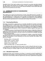
One-Dimensional Golden Section Search
GOLD(Il,
A2, A3, A4, A5, Bl, B2, B3, B4, J5)
Mischke
This subroutine
will
search over
a
one-dimensional
unimodal
function
and
report
the
largest ordinate
found,
its
abscissa,
final
abscissas bound
in the
interval
of
uncertainty,
and
the

number
of
function
evaluations expended during
the
search.
The
subroutine requires
the
specification
of the
present interval
of
uncertainty,
the
frac-
tional reduction required
in the
interval
of
uncertainty
(or
bilateral tolerance
on
abscissa
of
the
extreme),
and
whether

or not a
convergence monitor printout
is
desired.
The
neces-
sary
number
of
function
evaluations
may be
predicted
from
N
= 1 +
2.08
In
—
when
the
fractional reduction
in
interval
of
uncertainty
F is
given,
or
N=

I
2.08
In
Xr
~
x
*\
V
a
J
+
when
the
bilateral tolerance
a on
abscissa
of
extreme
is
given.
See
Introduction
to
Computer-Aided
Design,
C.
Mischke, Prentice-Hall, 1968,
p. 64, or
Mathematical
Model

Building,
2nd
rev. ed.,
C.
Mischke, Iowa State University Press, 1980,
pp.
282-290.
CALLING
PROGRAM
REQUIREMENTS
Provide
a
subroutine
A5(X,Y)
which returns
the
ordinate
Y
when
the
abscissa
X is
ten-
dered.
Provide
the
equivalent
of the
following
statement: EXTERNAL

A5
CALL
LIST ARGUMENTS:
Il = O,
convergence monitor
will
not
print
= 1
convergence monitor
will
print
A2
=
XC
original
left-hand
abscissa
of
interval
of
uncertainty
A3 =
x
r
original right hand abscissa
of
interval
of
uncertainty

A4 =
fractional reduction
in
interval
of
uncertainty desired,
F,
entered positive
or
bilateral tolerance
on
abscissa
at
extreme,
0,
entered negative
A5
=
name
of the
one-dimensional unimodal function SUBROUTINE
Bl
=
y*,
extreme ordinate discovered during search (maximum)
B2
=
x*,
abscissa
of

extreme ordinate
B3 =
;ti,
final
left-hand abscissa
of
interval
of
uncertainty
B4 =
Jc
2
,
final
right-hand abscissa
of
interval
of
uncertainty
J5 =
N
9
number
of
function
evaluations expended during search
PREEMPTED
NAMES:
None
SIZE:

4264
bytes WATFIV compiler.
FIGURE
11.1
The
documentation
page
of
subroutine
GOLD.
77.5
QUADRATURE
Another numerical chore
is
integration. Fortunately, Simpson's
first
rule
is
simple,
robust,
and
surprisingly accurate.
It is
applied
two
panels
at a
time with equally
spaced ordinates.
A

parabola
is
passed through
the
three ordinate points
([11.5],
p.
79).
If h is the
ordinate spacing, then
for the
three abscissas
Jt
0
,
*i,
and
Jt
2
,
£
2
/(*)
dx
=
|[f(*
0
)
+
4f(

Xl
)
+/(X
2
)]
-
|^/
(4)
©
(11.15)
where
^
is in the
interval
(jc
0
,
X
2
).
The
right-hand term
is
Richardson's
error
term,
which
is
exact
for

some
^
which
is
generally unknown
a
priori.
When this two-panel,
three-ordinate operation
is
repeated
a
number
of
times
in the
interval
a,
b,
then
f
f(x)
dx
=
\
\f(
Xo
)
+
4/(^

1
)
+
2/(X
2
)
+
• •
•
a
*
+
4/(*
2
_
_
O
+/fe,)]
-^J
/
4
>fe)
(11.16)
^
U
i
= 1
where
n is the
number

of
applications
of the
two-panel ritual,
2n
is the
number
of
panels,
and
2n
+1
is the
number
of
function
evaluations. There
is
great merit
in
mak-
ing
the
number
of
panels
an
even number divisible
by 4. The
ordinate spacing

h is
given
by h = (b -
a}/(2n),
and so the
error
term becomes, removing
the
summation
sign,
^wMf"®
(1L17)
By
evaluating
the
integral using
n
2
applications,
then
again with
HI
applications,
from
Eq.
(11.17),
fe-fe)' <
iu8
>
from

which
77
1/4
p
1/4
"l
«1
/11
10\
n
2
=
ni
-TT
1
-HI
-^-
(11.19)
£L>n2
^*
where
A is the
tolerable error.
If
HI
is the
number
of
applications
of the

rule
in the
interval
a,
b and
n
2
is the
number
of
applications
in
another evaluation
in the
same
interval
a, b,
then
the
value
of the
integral
I is
I
=
In
1
+E
ni
=

I
n2
+E
n2
If
W
2
is
one-half
of
W
1
,
then combining
Eq.
(11.18)
with
the
above
equation
results
in
7
^
+
^15^
(1L20)
f
2
Example

/.
Evaluate
the
integral dx/x.
J
i
(a)
Using
two
applications
of
Simpson's rule, estimate
the
error
in
I
n
=
2
.
(b} For an
error
of the
magnitude 0.000
01,
estimate
the
number
of
applications necessary,

and
(c)
integrate
and
examine
the
error.
Solution,
(a)
Using
two
applications
of
Simpson's rule,
x
l/x
Mult.
1.00 1.000000000
1
1.000000000
1.25
0.800000000
4
3.200000000
1.50
0.666666667
2
1.333333333
1.75 0.571428571
4

2.285714286
2.00
0.500000000
1
0.500
QOQ
OOP
Z
=
8.319047619
From
the
first
part
of Eq.
(11.16),
L
=
2
=
^-
(8319
047
619)
-
0.693
253 968
For one
application
of

Simpson's rule,
x l/x
Mult.
1.00 1.000000000
1
1.000000000
1.50 0.666666667
4
2.666666667
2.00
0.500000000
1
0.500
OOP
OOP
Z
=
4.166666667
/^
1
=
M
(4.166
666
667)
-
0.694
444
445
From

the
second part
of Eq.
(11.20),
I
n
=
2 - L
=
i
0.693
253 968 -
0.694
444 445
n
=
2
~
15 " 15
-
-0.000
079
565
(b)
From
Eq.
(11.19),
JEL
1/4
0

-Q.QQQ
079
365
1/4
_
_
.
H
^
n
^
2
=
2
Q.QQQ
Ql
=336=>4
(c)
Using
four
applications,
x Ux
Mult.
1.000 1.000000000
1
1.000000000
1.125 0.888888889
4
3.555555556
1.250

0.800000000
2
1.600
OPP
PPP
1.375 0.727272727
4
2.909090903
1.500 0.666666667
2
1.333333333
1.625 0.615384615
4
2.461538462
1.750 0.571428571
2
1.142857143
1.875
0.533333333
4
2.133333333
2.0OP
P.5PPPPPPPP
1
P.5PP
PPP PPP
I =
16.635
7P8
73

I
n
=
4
=
^p-
(16.635
708 73) =
0.693
154 530
The
true value
of the
integral
is
In
2 =
0.693
147
181.
The
value
of
I
n
=
4
differs
by 1 in
the

fifth
decimal place. Furthermore,
we can
improve
I
n
=
4
using
Eq.
(11.20):
J-T
_i_
77 — 7
_i_
n
=
4
~
n
~
2
-/
—
/«
=
4 +
^n
=
4 —

J-n
=
4+
TZ
=
0.693
154 530 -
0.000
006 629 =
0.693
147 901
and we
have
six
correct digits,
a
bonus since
we
estimated
E
n
=
4
along
the
way.
The use of
Simpson's rule
to
evaluate

an
integral
is
both controllably accurate
and
relatively simple.
11.6
CHECKING
It is
useful
to
check intermediate results
on an
as-you-go basis
as
well
as
upon com-
pletion.
If
there
are one
hundred subtasks involved
in
completing
an
engineering
task,
ponder this:
If

your average reliability
in
performing each subtask correctly
is
0.99,
then
the
probability
of
performing them
in
sequence correctly
is
0.99
100
,
or
0.37.
How
does
one
improve such
a
performance?
One way is by
checking.
If the
hundred
steps
are

concatenated
to
reach
the
result, where
in the
chain
of
events
is a
mistake
most
wasteful
in
effort
because work
has to be
repeated? Early! When
do
most peo-
ple
think
of
checking?
At the
end. Checking steps
as
they
are
done, checking groups

of
steps,
and
checking
the
final
result
is an
appropriate
and
wise course
of
action.
11.6.1
Limiting-Case
Check
This method
of
checking
a
derived equation allows
the
parameters,
in
turn,
to
range
from
the
point

of
vanishing
to
increasing without upper bound.
Do the
results still
make
sense?
Do the
results contract
to a
previously known correct result? Making
sense
is a
necessary
but not
sufficient
condition.
11.6.2
Dimensional
Check
Equations should
be
dimensionally homogeneous. Apply
the
dimensional operator
dim()
to
every term
in an

equation, substituting
the
fundamental dimensions term
by
term. Remember that
the
result
of
applying
the
operator
to a
dimensionless term
is
unity.
Dimensional homogeneity
is a
necessary
but not
sufficient
condition.
11.6.3
Experience
Our
lifetime experience with similar things will suggest
"expected
relationships":
symmetries
of
certain

forms,
indirect
and
direct proportionalities,
and
nonlineari-
ties
of a
particular order, such
as
proportionality
to the
cube
of
some parameter.
All
these
little
tidbits
of
reality
from
prior contexts
can be
examined
for
applica-
bility
to the
case

at
hand. Congruence with experience
is a
necessary
but not
suffi-
cient condition.
11.6.4
Robustness
of
Assumptions
Deductions
from
first
principles
and
cause-effect-extent mathematical models
depend
on
assumptions such
as
"friction
is
negligible"
or
"radiation
is
secondary."
What
we are

really saying
is
that
the
result
will
be
useful
to our
purpose—that
is,
robust—even
if the
influences
of
friction
or
radiation
are
ignored.
The
mathematical
meaning
of the
word assumption does
not
fully
apply here,
nor
does

it
serve
us
well.
In
reality,
we
have made
a
decision
based
on an
experiential value judgment that act-
ing
on the
result
is
prudent
and
resources
are
risked
at a
very small, acceptable level.
Engineers should treat
all
such
"assumptions"
as the
decisions they really are.

It is
useful
to ask
• Was it
necessary
to
make this decision (assumption)?
• Has
embracing
it
hidden
an
important influence
of the
surroundings
on
matter
in
the
system
or
control region?
• Did I
qualify
my
result with
an
explicit statement
of
this decision

(assumption)?
• Is
this decision (assumption) defendable
at all
values
of the
parameters that
will
be
encountered?
• Did
this decision (assumption) make
the
model
sufficiently
incongruent with
nature
to
lose robustness?
Thoughtful
responses
to
questions such
as
these
can
help uncover sketchy work.
Engineers
are
responsible

for
all the
decisions they make, whether
by
commission
or
by
omission.
It is
prudent
to
list (call out)
all
such decisions (assumptions)
in the
design notebook,
and the
responses
to
queries such
as
those above
in the
check
steps,
so
that
the
original engineer
at a

later date,
or
another engineer
at any
time,
can
understand,
appreciate,
and
possibly challenge
them.
11.6.5
Experiment
Results
can be
verified
by
experiment.
In
order
to
check
a
spring rate formulation,
such
as
,.
<PG
K
~8D

3
N
a
we
express
it in
dimensionless
form,
Eq.
(11.10):
JL_
=
J_(A\
=
K
= rt-
GD
SN
a
\D/
1
Sn
2
and
check
the two
nuggets
of
reality,
KI

K
2
=
Ci
and
KI!
K*
=
C
2
,
which were
the
bases
for
the
evaluation
of the
partial derivatives
of Eq.
(11.9).
The
first
lends itself
to a
lin-
ear
plot
of the
form

KI
=
CiIn
2
.
Ideally this should lead
to a
straight data string
on a
plot
of
Tii
versus
1/Ti
2
which lines
up
with
the
origin.
If one has
several springs which
differ
in
turns count only, placing known weights
on the
spring
and
measuring
the

deflection
with
a
dial indicator
can
supply some data points.
If
a
least-squares
fit of the
form
TCI
= a +
b/n
2
misses
the
origin,
has the
origin really
been missed?
There
are
statistical methods
for
saying that with
the
data
you
have,

the
origin
has
been
hit
(statistically)
or
missed (statistically)
and
quantifying
the
level
of risk in
believing
either.
For
example,
the
number
of
dead turns
N
d
comes
from
the
equation
N
t
=

N
d
+
N
a
.
The
number
of
dead turns
N
d
may not be
precisely
2,
depending
on how the
squared
and
ground
end
turns
are
actually formed.
The
determination
of
N
0
appears

to be a
counting procedure; that
is,
N
a
=
N
1
-
N
d
=
N
t
-2
implies great precision, except that
the
number
2 can be
suspect.
The
second experimental check
on
KI
=
C
2
K*
can be
done

on a
log-log
plot.
The
final
form
constant
C in Eq.
(11.10)
can be
found
from
the
experimental
data,
and
again, statistical methods
will
develop
the
chances that
C is
1/8.
Notice that
the
economy
of
effort
of
Sec. 11.2

is
used
to
make
an
experimental
check
one of
least
cost.
An
equation that
is an old
familiar friend, when applied out-
side
its
domain
of
validity, can't play
the
game well,
or at
all.
The
experimental check
can
detect this.
11.6.6
Alternative Method
of

Derivation
If
one is
truly
at
"the cutting edge,"
one
rejoices
at
achieving
a
result,
and
urging
a
second approach,
say an
energy method,
may not be
helpful. Nevertheless,
we are
rarely
at the
edge,
and an
alternative approach
is a
possible
and
useful

method
of
check.
For
example,
an
analog equation
can be
found.
11.6.7
Have
a
Colleague
Check
Your
Work
Often,
a
colleague
was
educated
at a
different
school
by a
different
faculty
using dif-
fering
emphases

and
methodologies. Some
of
these
may not be
familiar
to
you,
or of
first
choice. Having
a
colleague check brings
not
only
a
fresh
viewpoint
but a
dif-
ferent
ensemble
of
experience
to the
problem. While
a
challenge
to
some

of
your
decisions
may
result,
it
should
be
welcomed
in the
pursuit
of
soundness
and
com-
pleteness
of
analysis
and
documentation.
11.6.8
The
Insufficiency
of
Checking Methods
Methods
of
checking
are
directed toward verification

of
matters
of
mathematical
necessity
but not
sufficiency.
Additionally,
the
limiting-case check, dimensional
check,
experience check,
and
assumptions check
will
not
uncover
an
error
such
as in
the 8 of the
spring example.
The
experimental check
can,
the
alternative method
check
may,

and the
colleague check might detect
it.
Methods
of
checking
are
ways
of
detecting troubles.
In
themselves they
do not
rectify
troubles. Being unable
to
assure
infallibility,
engineers check, check,
and
check
again.
11.6.9
Checking
the
Problem-Solving Strategy
Failure
to
achieve
a

solution
or
ineffective
progress
in the
pursuit
of a
solution
can
be
traceable
to
problem-solving methodology. Previously identified checks were
focused
on
technical matters, usually mathematical modeling. Problem-solving
strategies
are
more global, more qualitative,
and
less tangible.
The
following ideas
and
questions
can be
useful
in
encouraging
a

healthy skepticism.
There
are
three clearly identifiable steps
in
problem solving:
(1)
defining
the
problem,
(2)
planning
its
treatment,
and (3)
executing
the
plan.
There
are two
more
steps which
are not
sequential,
but are
woven into
defining,
planning,
and
executing

as
necessary. They
are
also
the
final
two
steps
following
the
completion
of the
exe-
cution step. These
are (4)
checking
and (5)
learning
and
generalizing.
In
more detail,
the
steps consist
of
asking
the
following questions:
Defining
the

Problem
•
What
is the
real problem
or
issue?
•
What questions
are to be
answered?
•
What
are the
pertinent
facts?
• If
several problems
are
present, which should
be
addressed
first?
Planning
Its
Treatment
• How can I
solve
the
problem?

•
What fundamental principles apply?
•
What general truths will help toward
a
solution?
•
What
is my
plan
to
move
from
what
is
known
to
what
I
want?
• Is my
plan
sufficiently
complete
for
execution?
Has any
other work been done
on
this

problem?
Executing
the
Plan
•
What
is the
result
of my
plan?
• How do I get a
useful
result
from
the
principle applied?
•
Where
am I
with respect
to my
plan?
Checking
• Is my
work correct
in
every detail?
• Are
assumptions (decisions) reasonable?
•

Have
I
considered
all
important factors?
• Do the
results make good sense?
•
Have
I
applied
all
methods
of
checking?
Learning
and
Generalizing
•
What have
I
found
out?
•
What does
the
result tell
me
about
the

answer
to the
original problem?
•
What does
the
result mean,
and
what
is its
interpretation
in
common terms?
• How may my
results have
been
affected
by my
assumptions (decisions)?
• Is the
result good enough
to act
upon,
or
must
the
solution
be
refined?
In

moments
of
doubt
as to
what
to do
next,
ask
•
What
do I
really want
to
know?
•
What
am I
doing now?
•
Why?
•
Will
it
help?
All
this
is a
demonstration
of the
sagacity

of the
adage,
"There
are no
right answers,
only
right questions."
11.6.10
Checking
Cause-Effect-Extent
Models
Engineers tend
to be
self-sufficient
in
mastering cause-effect-extent models
of
sys-
tem/surroundings
interactions. This
in
turn leads them
to
rarely check
to see if
some relevant caveat
has
been
ignored.
For

example, changes
in
system internal
energy
are
those that occur
in the
absence
of
gravitation, motion, charge, mag-
netism,
and
capillarity.
If
internal energy
is a
consideration,
one
should check
to be
sure that these things
are
absent, inconsequential
in
magnitude,
or
accounted
for
in
some other way. Since this kind

of
information
is
scattered
in
many books
on
various subjects,
it can be
helpful
to
consult Ref.
[11.6],
which treats
more
than
a
hundred
effects
by
providing descriptions, illustrations, magnitude relations,
and
references.
11.6.11
Checking
Personal
Competence
There
are
times when every engineer

is "in
over
his or her
head"
and
outside
his or
her
personal knowledge
and
experience base. This happens occasionally because
no one can
predict where
a
solution
will
lead.
Engineers
do not
like
to
talk about
this.
The
best remedy
is
knowing when
to
seek help,
or the

resources
to
acquire
that help.
11.6.12
The
Final
Adequacy
Assessment
as a
Final
Check
An
adequacy assessment (Sec. 5.2) consists
of
those cerebral
and
empirical steps
that convince
the
designer that
the
specification
set
represents
a
robust design.
The
recommended step before "turning work
in" is a

final
adequacy assessment.
It
should begin
not
with what
is in
your head,
but
with information taken directly
from
the
report
and
drawings that
will
leave your desk.
Engineers
think
in
terms
of
sig-
nificant
attributes
(a
midrange length,
a
smallest diameter, etc.). These should
not be

remembered,
but
reconstructed
from
your specifications.
If you
have
been
thinking
in
terms
of,
say, active spring turns,
and you
have
entered
that
in the
spring maker's
form
blank
for
total turns,
you
will
set in
motion mass production
of
springs that
are

not
what
you had in
mind.
By
starting
the
final
adequacy assessment check with
what
leaves your desk,
you can
catch these kinds
of
errors.
Define
the
problem
Plan
its
treatment
What
is the
real problem
or
issue?
How can I
solve
the
problem?

What
questions
are to be
What fundamental principles apply?
answered?
What general truths
will
help
What
are the
pertinent facts? toward
a
solution?
If
several problems
are
present,
What
is my
plan
to
move from what
which
should
I
attack first?
is
known
to
what

I
want?
A
Is my
plan sufficiently complete
for
execution?
Has any
other work
been done
on
this
problem?
PROBLEM SOLVING
'
•
Define
the
problem
•
Plan
its
treatment
'
I
•
Execute
the
plan
Execute

the
plan
What
is the
result
of my
plan?
How
do I get a
useful
conclusion from
the
principle
I
applied?
Where
am I
with respect
to
my
plan?
•Check
1
I
•
Learn
and
generalize
Learn
and

generalize Check
What
have
I
found out?
Is
work correct
in
every detail?
What
does
the
result
tell
me Are
assumptions reasonable?
about
the
answer
to the
Have
I
considered
all
important
original
problem? factors?
What
does
the

result mean
and
Does
the
result make good sense?
what
is its
interpretation
in
common terms?
How
may the
results have been
affected
by my
assumptions?
Is
the
result good enough
to
act on or
must
the
solution
be
refined?
Ask
often
What
do I

really want
to
know?
What
am I
doing now?
Why?
Will
it
help?
FIGURE
11.2 Some pertinent questions
to ask
oneself while solving problems.
The
check, learn
and
generalize steps
are to be
woven into
the
first
three,
and are the
last ones.
REFERENCES
11.1
C. R.
Mischke, Mathematical Model
Building,

2d
rev. ed., Iowa State University Press,
Ames,
1980.
11.2
A. D.
Dimarogonas,
"Origins
of
Engineering Design,"
in
Design
Engineering,
vol.
62,
Vibrations
in
Mechanical Systems
and the
History
of
Engineering, American Society
of
Mechanical
Engineers
Design Conference Plenary Session presentation, Albuquerque,
September
1993.
11.3
C. R.

Mischke,
An
Introduction
to
Computer-Aided Design, Prentice-Hall,
Englewood
Cliffs,
NJ.,
1968.
11.4
G. V.
Reklaitis,
A.
Ravindran,
and K. M.
Ragsdell, Engineering Optimization,
Wiley-
Interscience,
New
York, 1983.
11.5
B.
Carnahan,
H. A.
Luther,
and J. O.
Wilkes, Applied Numerical Methods, John Wiley
&
Sons,
New

York, 1969.
11.6
C. F.
Hix, Jr.,
and R. P.
Alley, Physical Laws
and
Effects,
John
Wiley
&
Sons,
New
York,
1958.