Sổ tay tiêu chuẩn thiết kế máy P19 ppt

CHAPTER
15
INSTABILITIES
IN
BEAMS
AND
COLUMNS
Harry
Herman
Professor
of
Mechanical
Engineering
New
Jersey
Institute
of
Technology
Newark,
New
Jersey
15.1 EULER'S FORMULA
/
15.2
15.2
EFFECTIVE LENGTH
/
15.4
15.3
GENERALIZATION
OF THE

PROBLEM
/
15.6
15.4
MODIFIED BUCKLING FORMULAS
/
15.7
15.5
STRESS-LIMITING CRITERION
/
15.8
15.6 BEAM-COLUMN ANALYSIS
/
15.12
15.7
APPROXIMATE METHOD
/15.13
15.8 INSTABILITY
OF
BEAMS
/
15.14
REFERENCES
/15.18
NOTATION
A
Area
of
cross section
B(n)

Arbitrary
constants
c(h)
Coefficients
in
series
c(y),
c(z) Distance
from
y and z
axis, respectively,
to
outermost compressive
fiber
e
Eccentricity
of
axial load
P
E
Modulus
of
elasticity
of
material
E(t)
Tangent modulus
for
buckling
outside

of
elastic range
F(x)
A
function
of x
G
Shear modulus
of
material
h
Height
of
cross section
H
Horizontal (transverse) force
on
column
7
Moment
of
inertia
of
cross section
7(y),
I(z)
Moment
of
inertia with respect
to y and z

axis, respectively
/
Torsion constant; polar moment
of
inertia
k
2
PIEI
K
Effective-length
coefficient
K(Q)
Spring constant
for
constraining spring
at
origin
K(T,
O),
K(T,
L)
Torsional spring constants
at x =
O,
L,
respectively
/
Developed length
of
cross section

L
Length
of
column
or
beam
L
eff
Effective
length
of
column
M,
M'
Bending moments
M(O),
M(L),
M
mid
Bending moments
at x =
O,
L,
and
midpoint, respectively
M(0)
cr
Critical moment
for
buckling

of
beam
M
tr
Moment
due to
transverse load
M(v),
M(z)
Moment about
y and z
axis, respectively
n
Integer; running index
P
Axial load
on
column
F
cr
Critical axial load
for
buckling
of
column
r
Radius
of
gyration
R

Radius
of
cross section
s
Running coordinate, measured
from
one end
t
Thickness
of
cross section
T
Torque about
x
axis
x
Axial coordinate
of
column
or
beam
y,
z
Transverse coordinates
and
deflections
Y
Initial
deflection (crookedness)
of

column
y
tr
Deflection
of
beam-column
due to
transverse load
TI
Factor
of
safety
o
Stress
c|>
Angle
of
twist
As the
terms beam
and
column imply, this chapter deals with members whose cross-
sectional dimensions
are
small
in
comparison with their lengths. Particularly,
we are
concerned with
the

stability
of
beams
and
columns whose axes
in the
undeformed
state
are
substantially straight. Classically, instability
is
associated with
a
state
in
which
the
deformation
of an
idealized, perfectly straight member
can
become arbi-
trarily
large. However, some
of the
criteria
for
stable design which
we
will

develop
will
take into account
the
influences
of
imperfections such
as the
eccentricity
of the
axial
load
and the
crookedness
of the
centroidal axis
of the
column.
The
magnitudes
of
these imperfections
are
generally
not
known,
but
they
can be
estimated

from
manufacturing
tolerances.
For
axially
loaded columns,
the
onset
of
instability
is
related
to the
moment
of
inertia
of the
column cross section about
its
minor princi-
pal
axis.
For
beams, stability design requires,
in
addition
to the
moment
of
inertia,

the
consideration
of the
torsional
stiffness.
75.7
EULER'S FORMULA
We
will
begin with
the
familiar
Euler
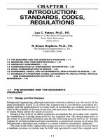
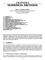
column-buckling problem.
The
column
is
ideal-
ized
as
shown
in
Fig.
15.1.
The top and
bottom ends
are
pinned; that
is, the
moments

at
the
ends
are
zero.
The
bottom
pin is
fixed
against translation;
the top pin is
free
to
move
in the
vertical direction only;
the
force
P
acts along
the x
axis, which coincides
with
the
centroidal axis
in the
undeformed
state.
It is
important

to
keep
in
mind that
the
analysis which
follows
applies only
to
columns with cross sections
and
loads that
are
symmetrical about
the xy
plane
in
Fig. 15.1
and
satisfy
the
usual assumptions
of
linear beam theory.
It is
particularly important
in
this connection
to
keep

in
mind that
this
analysis
is
valid only when
the
deformation
is
such that
the
square
of the
slope
of
the
tangent
at any
point
on the
deflection curve
is
negligibly small compared
to
unity
(fortunately,
this
is
generally true
in

design
applications).
In
such
a
case,
the
familiar
differential
equation
for the
bending
of a
beam
is
applicable. Thus,
d
2
y
EI-^
=
M
(15.1)
For the
column
in
Fig.
15.1,
M
= -Py

(15.2)
We
take
E and
7
as
constant,
and let
JJ
=
*
(15.3)
Then
we
get,
from
Eqs.
(15.1),
(15.2),
and
(15.3),
0
+
^
=
°
<
15
-
4

>
FIGURE
15.1 Deflection
of a
simply
supported
column,
(a)
Ideal
simply supported column;
(b)
column-deflection curve;
(c)
free-body
diagram
of
deflected
segment.
The
boundary conditions
at x = O and x = L are
XO)=XL)
= O
(15.5)
In
order that Eqs. (15.4)
and
(15.5) should have
a
solution

y(x)
that
need
not be
equal
to
zero
for all
values
of
x, k
must take
one of the
values
in Eq.
(15.6):
fcCO
=
-^
n
=
l,2,3,
(15.6)
l_j
which
means that
the
axial load
P
must take

one of the
values
in Eq.
(15.7):
P(n)
=
H
^f
7
«
=
1,2,3,
(15.7)
For
each value
of
n,
the
corresponding nonzero solution
for y is
y(rc)
=
#(rc)
sin
(^
j
n
=
1,2,3,
(15.8)

\
L
/
where
B(ri)
is an
arbitrary constant.
In
words,
the
preceding results state
the
following: Suppose that
we
have
a
per-
fectly
straight prismatic column with constant properties over
its
entire length.
If the
column
is
subjected
to a
perfectly axial load, there
is a set of
load values, together
with

a set of
sine-shaped deformation curves
for the
column axis, such that
the
applied moment
due to the
axial load
and the
resisting internal moment
are in
equi-
librium
everywhere along
the
column,
no
matter what
the
amplitude
of the
sine
curve
may be.
From
Eq.
(15.7),
the
smallest load
at

which such deformation occurs,
called
the
critical
load,
is
P^
(15-9)
This
is the
familiar
Euler
formula.
15.2
EFFECTIVELENGTH
Note that
the
sinusoidal shape
of the
solution
function
is
determined
by the
differ-
ential equation
and
does
not
depend

on the
boundary conditions.
If we can
find
a
segment
of a
sinusoidal curve that satisfies
our
chosen boundary conditions and,
in
turn,
we can
find
some segment
of
that curve which matches
the
curve
in
Fig. 15.1,
we
can
establish
a
correlation between
the two
cases. This notion
is the
basis

for the
"effective-length"
concept. Recall that
Eq.
(15.9)
was
obtained
for a
column with
both ends simply supported (that
is, the
moment
is
zero
at the
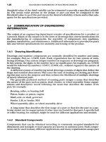
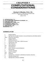
ends). Figure 15.2
illustrates columns
of
length
L
with various idealized
end
conditions.
In
each case,
there
is a
multiple
of L, KL,
which

is
called
the
effective
length
of the
column
L
e
ff,
that
has a
shape which
is
similar
to and
behaves like
a
simply supported column
of
that length.
To
determine
the
critical loads
for
columns whose
end
supports
may be

idealized
as
shown
in
Fig. 15.2,
we can
make
use of Eq.
(15.9)
if we
replace
L by KL,
with
the
appropriate value
of K
taken
from
Fig. 15.2. Particular care
has to be
taken
to
distinguish between
the
case
in
Fig.
15.2c,
where both ends
of the

column
are
secured against rotation
and
transverse translation,
and the
case
in
Fig.
15.2e,
where
the
ends
do not
rotate,
but
relative transverse movement
of one end of the
column
with
respect
to the
other
end is
possible.
The
effective
length
in the
first

case
is
half
that
in the
second case,
so
that
the
critical load
in the
first
case
is
four
times that
in
the
second case.
A
major
difficulty
with
using
the
results
in
Fig. 15.2
is
that

in
real
problems
a
column
end is
seldom perfectly
fixed
or
perfectly
free
(even approxi-
mately)
with regard
to
translation
or
rotation.
In
addition,
we
must remember that
the
critical load
is
inversely proportional
to the
square
of the
effective

length. Thus
a
change
of 10
percent
in
L
e
ff
will
result
in a
change
of
about
20
percent
in the
criti-
cal
load,
so
that
a
fair
approximation
of the
effective
length produces
an

unsatisfac-
tory approximation
of the
critical load.
We
will
now
develop more general
results
that
will
allow
us to
take into account
the
elasticity
of the
structure surrounding
the
column.
FIGURE
15.2
Effective
column lengths
for
different
types
of
support,
(a)

Simply
supported,
K =
I;
(b)
fixed-free,
K = 2; (c)
fixed-fixed,
K =
1
A;
(d)
fixed-pinned,
K =
0.707;
(e)
ends nonro-
tating,
but
have transverse translation.
75.3 GENERALIZATION
OF THE
PROBLEM
We
will
begin with
a
generalization
of the
case

in
Fig.
15.2e.
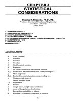
In
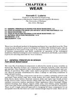
Fig. 15.3,
the
lower
end is no
longer
free
to
translate,
but
instead
is
elastically constrained.
The
differen-
tial equation
is
EI^
= M =
M(O)
+
PO(O)
-y] +
Hx
(15.10)
Here
H, the

horizontal force
at the
origin,
may be
expressed
in
terms
of the
deflec-
tion
at the
origin
y(O)
and the
constant
of the
constraining spring
K(Q):
H
=
-K(0)y(0)
(15.11)
M(O)
is the
moment which prevents rotation
of the
beam
at the
origin.
The

moment
which
prevents rotation
of the
beam
at the end x = L is
M(L).
The
boundary condi-
tions
are
*«-«
^=»
^"
<**>
The
rest
of the
symbols
are the
same
as
before.
We
define
k as in Eq.
(15.3).
As in the
case
of the

simply supported column, Eqs.
(15.10),
(15.11),
and
(15.12)
have solutions
in
which
y(x)
need
not be
zero
for all
values
of
x,
but
again these solutions occur only
for
certain values
of kL.
Here
these values
of kL
must
satisfy
Eq.
(15.13):
[2(1
- cos kL) - kL sin

kL]L
3
K(0)
+
EI(kL)
3
sin kL =
O
(15.13)
The
physical interpretation
is the
same
as in the
simply supported case.
If we
denote
the
lowest value
of kL
that
satisfies
Eq.
(15.13)
by
(A:L)
cr
,
then
the

column buckling
load
is
given
by
EI(kL)
2
cr
Per=
\2
(15.14)
FIGURE 15.3 Column with ends
fixed
against rotation
and an
elastic
end
constraint
against transverse
deflection,
(a)
Undeflected
column;
(b)
deflection curve;
(c)
free-
body diagram
of
deflected segment.

Since
the
column under consideration here
has
greater resistance
to
buckling than
the
case
in
Fig.
I5.2e,
the
(kL)
cr
here will
be
greater than
n.
We can
therefore evalu-
ate Eq.
(15.13)
beginning with
kL =
n
and
increasing
it
slowly until

the
value
of the
left
side
of Eq.
(15.13)
changes sign. Since
(kL)
CT
lies between
the
values
of kL for
which
the
left
side
of Eq.
(15.13)
has
opposite signs,
we now
have bounds
on
(kL)
CI
.
To
obtain improved bounds,

we
take
the
average
of the two
bounding values, which
we
will designate
by
(&L)
av
.
If the
value
of the
left
side
of Eq.
(15.13)
obtained
by
using
(kL)
av
is
positive (negative), then
(kL\
T
lies between
(fcL)

av
and
that value
of
kL for
which
the
left
side
of Eq.
(15.13)
is
negative (positive). This process
is
contin-
ued, using
the
successive values
of
(kL)
av
to
obtain improved bounds
on
(A:L)
cr
,
until
the
desired accuracy

is
obtained.
The
last
two
equations
in Eq.
(15.12)
imply perfect rigidity
of the
surrounding
structure with respect
to
rotation.
A
more general result
may be
obtained
by
taking
into account
the
elasticity
of the
surrounding structure
in
this respect. Suppose that
the
equivalent torsional spring constants
for the

surrounding structure
are
K(T,
O)
and
K(T,
L) at x = O and x = L,
respectively.Then
Eq.
(15.12)
is
replaced
by
XL)
= O
M(O)
=
K(T,
O)
^jJb-
(15.15)
M(L)
=
-K(T,
L)
^p-
Proceeding
as
before, with
Eq.

(15.15)
replacing
Eq.
(15.12),
we
obtain
the
following
equation
for kL:
l\
L3
IK(TM
+
K(Ti\\K(m
I
^K(O)K(T,
O)K(T,
p]
{[EI(kL)
3
\
[K(T
'
0
'
+
K(T
'
L

'
]K(()
>~[
(E/)
2
(fcL)
3
J
[AT(O)L
2
I
I
LK(T,
O)K(T,
L)I
[
EI(kL)~\]
.
1T
+
/,
'
+
„./.
,\
—^-
-
—T—
L
\

sm
kL
I
(kL)
J [
EI(kL)
J [ L JJ
+
\K(T,
O)
+
K(T,
L) -
LJrIJ
[K(T,
O)
+
K(T,
L)]AT(O)]
cos kL
i
L-Zi^KL,)
J J
+
2
^,O)WOHML)]( „„,,.„
(15
.
16)
The

lowest value
of kL
satisfying
Eq.
(15.16)
is the
(kL)
cl
to be
substituted
in Eq.
(15.14)
in
order
to
obtain
the
critical load.
Here
there
is no
apparent good guess
with
which
to
begin computations. Considering
the
current accessibility
of
comput-

ers,
a
convenient approach would
be to
obtain
a
plot
of the
left
side
of Eq.
(15.16)
for
0<kL<n,
and if
there
is no
change
in
sign, extend
the
plot
up to kL =
2n,
which
is
the
solution
for the
column with

a
perfectly rigid surrounding structure
(Fig.
15.2c).
However,
see
also Chap.
4.
75.4
MODIFIEDBUCKLINGFORMULAS
The
critical-load formulas developed above provide satisfactory values
of the
allow-
able load
for
very slender columns
for
which buckling,
as
manifested
by
unaccept-
ably
large deformation,
will
occur within
the
elastic range
of the

material.
For
more
massive columns,
the
deformation
enters
the
plastic region (where strain
increases
more rapidly with stress) prior
to the
onset
of
buckling.
To
take into account this
change
in the
stress-strain relationship,
we
modify
the
Euler
formula.
We
define
the
tangent
modulus

E(f)
as the
slope
of the
tangent
to the
stress-strain curve
at a
given
strain. Then
the
modified formulas
for the
critical load
are
obtained
by
substituting
E(f)
for E in Eq.
(15.9)
and Eq.
(15.13)
plus
Eq.
(15.14)
or Eq.
(15.16)
plus
Eq.

(15.14).
This
will
produce
a
more accurate prediction
of the
buckling load. However,
this
may not be the
most desirable design approach.
In
general,
a
design which will
produce plastic deformation under
the
operating load
is
undesirable.
Hence,
for a
column
which
will
undergo plastic deformation prior
to
buckling,
the
preferred

design-limiting
criterion
is the
onset
of
plastic deformation,
not the
buckling.
15.5
STRESS-LIMITING
CRITERION
We
will
now
develop
a
design criterion which will enable
us to use the
yield strength
as
the
upper bound
for
acceptable design regardless
of
whether
the
stress
at the
onset

of
yielding precedes
or
follows
buckling.
Here
we
follow
Ref.
[15.1].
This
approach
has the
advantage
of
providing
a
single bounding criterion that holds irre-
spective
of the
mode
of
failure.
We
begin
by
noting that,
in
general, real columns
will

have
some imperfection, such
as
crookedness
of the
centroidal axis
or
eccentricity
of
the
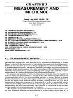
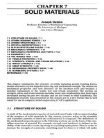
axial load. Figure 15.4 shows
the
difference
between
the
behavior
of an
ideal,
perfectly
straight column subjected
to an
axial load,
in
which case
we
obtain
a
dis-
tinct
critical point,

and the
behavior
of a
column with some imperfection.
It is
clear
from
Fig. 15.4 that
the
load-deflection curve
for an
imperfect column
has
no
distinct critical point. Instead,
it has two
distinct regions.
For
small axial loads,
the
deflection increases slowly with load. When
the
load
is
approaching
the
critical
value
obtained
for a

perfect column,
a
small increment
in
load produces
a
large
change
in
deflection. These
two
regions
are
joined
by a
"knee."
Thus
the
advent
ofL
buckling
in a
real column corresponds
to the
entry
of the
column into
the
second,
above-the-knee,

load-deflection region.
A
massive column will reach
the
stress
at
the
yield point prior
to
buckling,
so
that
the
yield strength
will
be the
limiting crite-
rion
for the
maximum allowable load.
A
slender column
will
enter
the
above-the-
TRANSVERSE
DEFLECTION
FIGURE 15.4 Typical load-deflection curves
for

ideal
and
real
columns.
IDEAL
COLUMN
IMPERFECT COLUMN
knee region prior
to
reaching
the
stress
at the
yield point,
but
once
in the
above-the-
knee region,
it
requires only
a
small increment
in
load
to
produce
a
sufficiently
large

increase
in
deflection
to
reach
the
yield point. Thus
the
corresponding yield load
may
be
used
as an
adequate
approximation
of the
buckling load
for a
slender
col-
umn as
well.
Hence
the
yield strength provides
an
adequate design bound
for
both
massive

and
slender columns.
It is
also important
to
note that,
in
general, columns
found
in
applications
are
sufficiently
massive that
the
linear theory developed here
is
valid within
the
range
of
deflection that
is of
interest.
Application
of Eq.
(15.1)
to a
simply supported imperfect column with constant
properties

over
its
length yields
a
modification
of Eq.
(15.4). Thus,
^
+
tfy
=
k\e-Y)
(15.17)
where
e =
eccentricity
of the
axial load
P
(taken
as
positive
in the
positive
y
direc-
tion)
and Y =
initial deflection (crookedness)
of the

unloaded column.
The x
axis
is
taken through
the end
points
of the
centroidal axis,
so
that
Eq.
(15.5) still holds
and
Yis
zero
at the end
points. Note that
the
functions
in the
right side
of Eq.
(15.8)
form
a
basis
for a
trigonometric (Fourier) series,
so

that
any
function
of
interest
may be
expressed
in
terms
of
such
a
series. Thus
we can
write
Y=
Y
c
(n)
sin
^
(15.18)
n
=
l
L
where
C(H)
=
-ff

Y(X)Sm^dX
(15.19)
L
J
0
Li
The
solution
for the
deflection
y in Eq.
(15.17)
is
given
by
^
f
.
.
4e~\
sin
(nnx/L)
y
=
Py
\c(ri)-
rz7r/
/r\2
P1
(15.20)

n
=
i
L
nn
J
[EI(nnlL)
2
-P]
^
'
The
maximum deflection
v
max
of a
simply supported column
will
usually (except
for
cases with
a
pronounced
and
asymmetrical initial deformation
or
antisymmetrical
load eccentricity) occur
at the
column midpoint.

A
good approximation (probably
within
10
percent)
of
y
max
in the
above-the-knee region that
may be
used
in
deflection-
limited column design
is
given
by the
coefficient
of the
first
term
in Eq.
(15.20):
P[c(l)
~(4e/n)}
ymax
~
EI(KlL)
2

-P
^
D
-
Z1;
The
maximum bending moment will also usually occur
at the
column midpoint
and
at
incipient yielding
is
closely approximated
by
M
mM
=
p{
g
-y
m
.
d
+
[f-c(l)]
[£/(7t/
f
)2
_

p]
}
(15.22)
The
immediately preceding analysis deals with
the
bending moment about
the z
axis (normal
to the
paper). Clearly,
a
similar analysis
can be
made with regard
to
bending about
the y
axis (Fig.
15.1).
Unlike
the
analysis
of the
perfect column, where
it is
merely
a
matter
of

finding
the
buckling load about
the
weaker axis,
in the
present approach
the
effects
about
the two
axes interact
in a
manner familiar
from
analysis
of an
eccentrically loaded short strut.
We now use the
familiar
expression
for
combining direct axial stresses
and
bending stresses about
two
perpendicular
axes. Since there
is no
ambiguity,

we
will
suppress
the
negative sign associated with
compressive
stress:
P
M(
Z
)c(y)
M(y)c(
Z
)
°
=
A
+
/(Z)
+
I(y)
(15
'
23)
where
c(y)
and
c(z)
=
perpendicular distances

from
the z
axis
and y
axis, respectively
(these axes meet
the x
axis
at the
cross-section centroid
at the
origin),
to the
outer-
most
fiber
in
compression;^
=
cross-sectional area
of the
column;
and a =
total com-
pressive stress
in the
fiber
which
is
farthest removed

from
both
the y and z
axes.
For
an
elastic design limited
by
yield strength,
a is
replaced
by the
yield strength;
M(z)
in
the
right side
of Eq.
(15.23)
is the
magnitude
of the
right side
of Eq.
(15.22);
and
M(y)
is an
expression similar
to Eq.

(15.22)
in
which
the
roles
of the y and z
axes
interchange.
Usually,
in
elastic design,
the
yield strength
is
divided
by a
chosen
factor
of
safety
TI
to get a
permissible
or
allowable stress.
In
problems
in
which
the

stress increases
linearly
with
the
load, dividing
the
yield stress
by the
factor
of
safety
is
equivalent
to
multiplying
the
load
by the
factor
of
safety.
However,
in the
problem
at
hand,
it is
clear
from
the

preceding development that
the
stress
is not a
linear
function
of the
axial
load
and
that
we are
interested
in the
behavior
of the
column
as it
enters
the
above-the-knee region
in
Fig. 15.4.
Here
it is
necessary
to
multiply
the
applied axial

load
by the
desired
factor
of
safety.
The
same procedure applies
in
introducing
a
fac-
tor of
safety
in the
critical-load formulas previously derived.
Example
1. We
will
examine
the
design
of a
nominally straight column supporting
a
nominally concentric load.
In
such
a
case,

a
circular column cross section
is the
most reasonable choice, since there
is no
preferred direction.
For
this case,
Eq.
(15.23) reduces
to
P
Mc
,_
O=A
+
-T
W
For
simplicity,
we
will
suppose that
the
principal imperfection
is due to the
eccentric
location
of the
load

and
that
the
column crookedness
effect
need
not be
taken into
account,
so
that
Eq.
(15.22) reduces
to
M
-
=
P
{
e
+
(^)
(EW-P]]
&
Note that
for a
circular cross section
of
radius
R,

the
area
and
moment
of
inertia are,
respectively,
A=nff
and
/=^f
=
£
(3)
We
will
express
the
eccentricity
of the
load
as a
fraction
of the
cross-section radius.
Thus,
e =
e,R
(4)
Then
we

have,
from
Eqs.
(1)
through
(4),
_Z
4Pe
f
/4\
P \
cJaiiow-^+
A
[
L
+
(
n
)
[(EA
2
)/(4n)](n/L)
2
-Pj
w
Usually
P and L are
given,
a and E are the
properties

of
chosen material,
and 8 is
determined
from
the
clearances, tolerances,
and
kinematics involved,
so
that
Eq. (5)
is
reduced
to a
cubic
in A.
At the
moment, however,
we are
interested
in
comparing
the
allowable nominal
column stress
PIA
with
the
allowable stress

of the
material
a
a
u
ow
for
columns
of
dif-
ferent
lengths. Keeping
in
mind that
the
radius
of
gyration
r of a
circular cross sec-
tion
of
geometric radius
R is
R/2,
we
will
define
R
^

=
r
^=P
(6)
E
fallow
~
q
Then
Eq. (5) may be
written
as
p
= 1 +
4e
+
—r~2—/
ir\2—TT
(7)
F
n[n
2
pq(r/L)
2
-l]
v
>
The
first
term

on the
right
side
of Eq. (7) is due to
direct
compressive
stress;
the
sec-
ond
term
is due to the
bending moment produced
by the
load eccentricity;
the
third
term
is due to the
bending moment arising
from
the
column deflection. When
8 is
small,
p
will
be
close
to

unity unless
the
denominator
in the
third term
on the
right
side
of Eq. (7)
becomes
small—that
is, the
moment
due to the
column deflection
becomes large.
The
ratio
LIr,
whose reciprocal appears
in the
denominator
of the
third term,
is
called
the
slenderness
ratio.
Equation

(7) may be
rewritten
as a
quadratic
in p.
Thus,
Wf)
2
P
2
-
[(I
+
*0
Wf
)
2
+
ll
p
+
(1
+
48)
-
1
^-
=
O
(8)

\L,/
I
\L,/
J
K
We
will
take
for q the
representative value
of
1000
and
tabulate
1/p
for a
number
of
values
of LIr and e. To
compare
the
value
of
1/p
obtained
from
Eq. (8)
with
the

cor-
responding result
from
Euler's
formula,
we
will
designate
the
corresponding result
obtained
by
Euler's
formula
as
l//?
cr
and
recast
Eq.
(15.9)
as
i^
To
interpret
the
results
in
Table
15.1,

note that
the
quantities
in the
second
and
third
columns
of the
table
are
proportional
to the
allowable loads calculated
from
the
respective equations.
As
expected,
the
Euler
formula
is
completely inapplicable
when
LIr is 50.
Also,
as
expected,
the

allowable load decreases
as the
eccentricity
increases. However,
the
effect
of
eccentricity
on the
allowable load decreases
as the
slenderness ratio
LIr
increases.
Hence
when
LIr is
250,
the
Euler buckling load,
which
is the
limiting case
for
which
the
eccentricity
is
zero,
is

only about
2
percent
higher than when
the
eccentricity
is 2
percent.
TABLE
15.1
Influence
of
Eccentricity
and
Slenderness
Ratio
on
Allowable
Load
e
L/r
p~
l
P^
0.02
50
0.901 3.95
150
0.408
0.439

250
0.155 0.158
0.05
50
0.791 3.95
150
0.374
0.439
250
0.151 0.158
0.10
50
0.665
3.95
150
0.333
0.439
250
0.145 0.158
75.6
BEAM-COLUMNANALYSIS
A
member that
is
subjected
to
both
a
transverse load
and an

axial load
is
frequently
called
a
beam-column.
To
apply
the
immediately preceding stress-limiting criterion
to a
beam-column,
we
first
determine
the
moment distribution, say,
M
tr
,
and the
cor-
responding deflection, say,
y
tr
,
resulting
from
the
transverse load acting alone. Sup-

pose that
the
transverse load
is
symmetrical about
the
column midpoint,
and let
^tr,mid
and
M
tr
,
m
id
be the
values
of
Y
tr
and
M
tr
at the
column midpoint. Then
the
only
modifications
necessary
in the

preceding development
are to
replace
Y by
Y
+
Y
ir
in
Eqs.
(15.17)
and
(15.20),
and to
replace
Y
mid
by
Y
mid
+
y
tr(inid
and add
M
tr
,
mid
on the
right

side
of Eq.
(15.23).
If the
transverse load
is not
symmetrical, then
it is
necessary
to
determine
the
maximum moment
by
using
an
approach which will
now be
devel-
oped.
Note that,
at any
point,
x,
the
moment about
the z
axis
is
M(z)

=
P(e-y-Y)
+
M(Z)*
(15.24)
where
Y
includes
the
deflection
due to
M(z)
tr
.
M(y)
has the
same
form
as Eq.
(15.24),
but
with
the
roles
of
y and z
interchanged.
The
maximum stress
for any

given
value
of x is
given
by Eq.
(15.23).
We
seek
to
apply this equation
at
that value
of x
which
yields
the
maximum value
of
o.
A
method that
is
reasonably
efficient
in
locat-
ing
a
minimum
or

maximum
to any
desired accuracy
is the
golden-section search.
However, this method
is
limited
to
finding
the
minimum (maximum)
of a
unimodal
function,
that
is, a
function
which
has
only
one
minimum (maximum)
in the
interval
in
which
the
search
is

conducted.
We
therefore have
to
conduct some exploratory
calculation
to
find
the
stress
at,
say,
a
dozen points
on the
beam-column
in
order
to
locate
the
unimodal interval
of
interest within which
to
apply
the
golden-section
search.
The

actual number
of
exploratory calculations
will
depend
on the
individual
case.
For
example,
in a
simply supported case with
a
unimodal transverse moment,
there
is
clearly only
one
maximum. But,
in
general,
we
must check enough points
to
be
sure that
a
potential maximum
is not
overlooked.

The
golden-section search procedure
is as
follows:
Suppose that
we
seek
the
min-
imum
value
of
F(X)
in
Fig. 15.5 within
the
interval
D
(note that
if we
sought
a
maxi-
mum
in
Fig. 15.5,
we
would have
to
conduct

two
searches).
We
locate
two
points x(l)
and
x(2).
The
first
is
0.382D
from
the
left
end of the
interval;
the
second
is
0.382D
FIGURE 15.5 Finding
min
F(X)
in the
interval
D.
from
the
right end.

We
evaluate
F(X)
at the
chosen points.
If the
value
of
F(JC)
at
Jt(I)
is
algebraically smaller than
at
;t(2),
then
we
eliminate
the
subinterval between x(2)
and
the
right
end of the
search interval.
In the
oppositive event,
we
eliminate
the

subinterval
between
Jt(I)
and the
left
end.
The
distance
of
0.236D
between
x(l)
and
x(2)
equals 0.382
of the new
search
interval, which
is
0.61&D
overall.
Thus
we
have
already
located
one
point
at
0.382

of the new
search interval,
and we
have deter-
mined
the
value
of
F(X)
at
that point.
We
need only locate
a
point that
is
0.382
from
the
opposite
end of the new
search interval, evaluate
F(x)
at
that point,
and go
through
the
elimination procedure,
as

before,
to
further
reduce
the
search interval.
The
process
is
repeated until
the
entire remaining interval
is
small
and the
value
of
F(X)
at the two
points
at
which
it is
evaluated
is the
same within
the
desired accuracy.
The
preceding method

may run
into
difficulty
if the
function
F(X)
is flat,
that
is, if
F(x)
does
not
vary
over
a
substantial part
of the
search interval
or if
F(X)
happens
to
have
the
same value
at the two
points that
are
compared with each other.
The

first
case
is not
likely
to
occur
in the
types
of
problems under consideration here.
In the
second case,
we
calculate
F(X)
at
another point, near
one of the two
points
of
com-
parison,
and use the
newly
chosen point
in
place
of the
nearby original point. Refer-
ence [15.2] derives

the
golden-section search strategy
and
provides equations
(p.
289)
for
predicting
the
number
of
function
evaluations required
to
attain
a
specified
fractional
reduction
of
search interval
or an
absolute
final
search interval size.
15.7
APPROXIMATEMETHOD
The
reason
why we

devoted
so
much attention
to
uniform
prismatic column prob-
lems
is
that their solution
is
analytically simple,
so
that
we
could obtain
the
results
directly.
In
most other cases,
we
have
to be
satisfied with approximate formulations
for
computer
(or
programmable calculator) calculation
of the
solution.

The
finite-
element
method
is the
approximation method most
widely
used
in
engineering
at
the
present time
to
reduce problems dealing with continuous systems, such
as
beams
and
columns,
to
sets
of
algebraic equations that
can be
solved
on a
digital computer.
When there
is a
single independent variable involved

(as in our
case),
the
interval
of
interest
of the
independent variable
is
divided into
a set of
subintervals called
finite
elements.
Within each subinterval,
the
solution
is
represented
by an arc
that
is
defined
by a
simple
function,
usually
a
polynomial
of low

degree.
The
curve result-
ing
from
the
connected
arc
segments should have
a
certain degree
of
smoothness
(for
the
problems under discussion,
the
deflection curve
and its
first
derivative
should
be
continuous)
and
should approximate
the
solution.
An
effective

method
of
obtaining
a
good approximation
to the
solution
is
based
on the
mechanical energy
involved
in the
deformation process.
15.8
INSTABILITYOFBEAMS
Beams
that have rectangular cross sections with
the
thickness much smaller than
the
depth
are
prone
to
instability involving rotation
of the
beam cross section about
the
beam axis. This tendency

to
instability arises because such beams have
low
resistance
to
torsion about their axes.
In
preparation
for the
analysis
of
this problem, recall that
for
a
circular cylindrical member
of
length
L and
radius
R,
subjected
to an
axial
torque
T, the
angle
of
twist
§
is

given
by
O=T!
<
15
-
25
)
where
G =
shear modulus
and / =
polar moment
of
inertia
of the
cross section.
For
noncircular
cross sections,
the
form
of the
right side
of Eq.
(15.25) does
not
change;
the
only change

is in the
expression
for J, the
torsion constant
of the
cross
section.
If
the
thickness
of the
cross section,
to be
denoted
by t, is
small
and
does
not
vary
much,
then
/ is
given
by
3J=l?ds
(15.26)
J
o
where

s =
running coordinate measured
from
one end of the
cross section
and / =
total developed length
of the
cross section. Thus,
for a
rectangular cross section
of
depth
h,
/
=
-y
(15.27)
Clearly,
/
decreases rapidly
as t
decreases.
To
study
the
effect
of
this circumstance
on

beam stability,
we
will
examine
the
deformation
of a
beam with rectangular
cross
section subjected
to end
moments M(O), taking into account rotation
of the
cross
section about
the
beam axis.
The
angle
of
rotation
§
is
assumed
to be
small,
so
that
sin
(|)

may be
replaced
by
(})
and cos
<|)
by
unity.
The
equations
of
static equilibrium
may be
written
from
Fig. 15.6, where
the
moments
are
shown
as
vectors, using
the
right-hand rule:
-M'(z)
+
M(O)
= O
M'(y)
+

M(0)<|>
= O
(15.28)
dT
dM\z)
+
_Q
ax
ax
VIEW
B-B OF
ELEMENT
dx
FIGURE 15.6 Instability
of
beams,
(a)
Segment
of a
beam with applied moment M(O)
at the
ends;
(b)
cross section
of
undeformed
beam;
(c)
cross section
after

onset
of
beam instability;
(d)
top
view
of
undeformed
differential
beam element;
(e)
the
element
after
onset
of
instability.
These, combined with
Eq.
(15.25)
and the
standard moment-curvature relation
as
given
by Eq.
(15.1),
lead
to the
defining
differential equation (15.29)

for the
angle
§\
GJ
44
+
M
2
(0)(|)
-~r^
-
-^T-T
=
O
(15.29)
dx
2
^
'
Y
\_EI(y)
EI(z)
J
v
'
Suppose that
the end
faces
of the
beam

are
fixed
against rotation about
the x
axis.
Then
the
boundary conditions
are
(I)(O)
=
<|>(L)
= O
(15.30)
Noting
the
similarity between
Eq.
(15.4)
with
its
boundary
conditions
[Eq.
(15.5)]
and Eq.
(15.29) with
its
boundary conditions [Eq.
(15.3O)],

the
similarity
of the
solu-
tions
is
clear. Thus
we
obtain
the
expression
for
M(0)
cr
:
i^-^^tt]
<-"»
It
may be
seen
from
Eq.
(15.31)
that
if the
torsion constant
/ is
small,
the
critical

moment
is
small.
In
addition,
it may be
seen
from
the
bracketed term
in Eq.
(15.31)
that
as the
cross section approaches
a
square shape,
the
denominator becomes small,
so
that
the
critical moment becomes very large.
The
disadvantage
of a
square cross
section
is, of
course, well known.

To
demonstrate
it
explicitly,
we
rewrite
the
expres-
sion
for
stress
in a
beam with rectangular cross section
t by
h:
M(h/2)
O
=
^JU
<
1532
)
in
the
form
*-w
"«
3
>
Thus,

for
given values
of M and a, the
cross-sectional area required decreases
as we
increase
h.
Hence
the
role
of Eq.
(15.31)
is to
define
the
constraint
on the
maximum
allowable
depth-to-thickness ratio.
The
situation
is
similar
for
flanged
beams.
Here
we
have obtained

the
results
for a
simple problem
to
illustrate
the
disadvantage
involved
and the
caution necessary
in
designing beams with thin-walled open cross
sections. Implicit
in
this
is the
advantage
of
using, when possible, closed cross sec-
tions, such
as box
beams, which have
a
high torsional
stiffness.
As we
have seen, when
the
applied moment

is
constant over
the
entire length
of
the
beam,
the
problem
of
definition
and its
solution have
the
same
form
as for the
column-buckling
problem.
We can
also have similar types
of
boundary conditions.
The
boundary conditions used
in Eq.
(15.30)
correspond
to a
simply supported col-

umn.
If
dyldx
and
dzldx
are
equal
to
zero
at x = O for all y and z,
then
dty/dx
is
equal
to
zero
at x =
O.
If
this condition
is
combined with
c|>(0)
=
O,
then
we
have
the
equiva-

lent
of a
clamped column end.
Hence
we can use
here
the
concept
of
equivalent
beam length
in the
same manner
as we
used
the
equivalent column length before.
In
case
a
beam
is
subjected
to
transverse loads,
so
that
the
applied moment varies with
x, the

problem
is
more complex.
For the
proportioning
of flanged
beams, Ref.
[15.3]
should
be
used
as a
guide. This reference deals with structural applications,
so
that
the
size range
of
interest dealt with
is
different
from
the
size range
of
interest
in
machine
design.
But the

underlying principles
of
beam stability
are the
same,
and
the
proportioning
of the
members should
be
similar.
Example
2. We
will
examine
the
design
of a
beam
of
length
L and
rectangular
cross section
t by h. The
beam
is
subjected
to an

applied moment
M (we
will
not use
any
modifying
symbols here, since there
is no
ambiguity), which
is
constant over
the
length
of the
beam.
As
noted previously,
the
required cross-sectional area
th
will
decrease
as h is
increased.
We
take
the
allowable stress
in the
material

to be a. The
calculated
stress
in the
beam
is not to
exceed this value. Thus,
M(h/2)
6M
1
6M
a
-^/12~
°-ltf
th
~~te
(1)
We
want
the
cross-sectional area
th as
small
as
possible.
Hence
h
should
be as
large

as
possible.
We
can, therefore, replace
the
inequality
in Eq. (1) by the
equality
-£
The
maximum value
of h
that
we can use is
subject
to a
constraint based
on Eq.
(15.31).
We
will
use a
factor
of
safety
T]
in
this connection. Thus,
^^{-am
Here

'<*>=£
'<»=£
'=f
<
4
>
Using
Eq.
(4),
we may
write
Eq. (3) as
(^W
(i)
2
[nwH
(5)
or,
from
Eq.
(2),
/
,n^rc
2£G
/
6M
Vr
1
]/6MV
(TlM)

2
<
W
^j
[lT[(^^|^)
(6)
Since
we
seek
to
minimize
th and
maximize
/z,
it may be
seen
from
Eqs.
(5) and (6)
that
the
inequality sign
may be
replaced
by the
equality sign
in
those
two
equations.

In Eq.
(6),
h is the
only unspecified quantity. Further, since
the
square
of
tlh
may be
expected
to be
small compared
to
unity,
we can
obtain substantially simpler approx-
imations
of
reasonable accuracy.
As a
first
step,
we
have
rw=
1+
(i)
2+
(i)
4+

-
^
If
we
retain only
the
first
two
terms
in the
right
side
of Eq.
(7),
we
have
n(EGY
12
F
1
/6M\
2
]/6MW6MV
w=—«r-
H^jj(^Ju^)
^
If
we
also neglect
the

square
of tlh in
comparison with unity,
we
obtain
r7i(6M)
2
(£G)
1/2
~|i/5
K
nLo'
J
^
as
a
reasonable
first
approximation. Thus
if we
take
the
factor
of
safety
r|
as
1.5,
we
have,

for a
steel member with
E = 30
Mpsi,
G
= 12
Mpsi,
and a = 30
kpsi,
r7i(36)[(30xlO*)(12xlO*)]
ia
M
2
I'"
,,JM
2
V*
h
=
[
(1.5)(30000)
~L\
=
8
'
6
H~)
(10)
This
is a

reasonable approximation
to the
optimal height
of the
beam cross section.
It may
also
be
used
as a
starting point
for an
iterative solution
to the
exact expres-
sion,
Eq.
(6).
For the
purpose
of
iteration,
we
rewrite
Eq. (6) as
_
f7t(6M)
2
F
EG

]
1/2
1
1/5
*
=
l
ULa
3
[l-[(6M)/(/z
3
a)]
2
J
)
(11)
The
value
of h
obtained
from
Eq. (9) is
substituted into
the
right side
of Eq.
(11).The
resultant value
of
h

thus obtained
is
then resubstituted into
the
right side
of Eq.
(11);
the
iterative process
is
continued until
the
computed value
of h
coincides with
the
value
substituted into
the
right side
to the
desired degree
of
accuracy. Having deter-
mined
h,
we can
determine
t
from

Eq.
(2).
REFERENCES
15.1
H.
Herman,
"On the
Analysis
of
Uniform Prismatic Columns,"
Transactions
of the
ASME, Journal
of
Mechanical
Design, vol.
103,1981,
pp.
274-276.
15.2
C. R.
Mischke, Mathematical Model Building,
2d
rev. ed., Iowa State University Press,
Ames, 1980.
15.3
Manual
of
Steel
Construction,

8th
ed.,
American Institute
of
Steel Construction,
New
York.