Sổ tay tiêu chuẩn thiết kế máy P20 pot

CHAPTER
16
CURVED
BEAMS
AND
RINGS
Joseph
E.
Shigley
Professor
Emeritus
The
University
of
Michigan
Ann
Arbor, Michigan
16.1 BENDING
IN THE
PLANE
OF
CURVATURE
/
16.2
16.2
CASTIGLIANO'S
THEOREM
/
16.2
16.3 RING SEGMENTS WITH
ONE

SUPPORT
/
16.3
16.4
RINGS WITH SIMPLE SUPPORTS
/16.10
16.5
RING SEGMENTS WITH FIXED ENDS
/
16.15
REFERENCES/16.22
NOTATION
A
Area,
or a
constant
B
Constant
C
Constant
E
Modulus
of
elasticity
e
Eccentricity
F
Force
G
Modulus

of
rigidity
/
Second moment
of
area (Table
48.1)
K
Shape constant (Table 49.1),
or
second polar moment
of
area
M
Bending moment
P
Reduced load
Q
Fictitious force
R
Force reaction
r
Ring radius
r
Centroidal ring radius
T
Torsional moment
U
Strain energy
V

Shear
force
W
Resultant
of a
distributed load
w
Unit distributed load
X
Constant
Y
Constant
y
Deflection
Z
Constant
y
Load angle
$
Span angle,
or
slope
a
Normal stress
6
Angular coordinate
or
displacement
Methods
of

computing
the
stresses
in
curved beams
for a
variety
of
cross
sections
are
included
in
this chapter. Rings
and
ring segments loaded normal
to the
plane
of
the
ring
are
analyzed
for a
variety
of
loads
and
span angles,
and

formulas
are
given
for
bending moment, torsional moment,
and
deflection.
16.1
BENDINGINTHEPLANEOFCURVATURE
The
distribution
of
stress
in a
curved member subjected
to a
bending moment
in the
plane
of
curvature
is
hyperbolic
([16.1],
[16.2])
and is
given
by the
equation
My

G=
A
,
r
(16.1)
Ae(r
-e-y)
^
'
where
r =
radius
to
centroidal axis
y
=
distance
from
neutral axis
e
=
shift
in
neutral axis
due to
curvature
(as
noted
in
Table 16.1)

The
moment
M is
computed about
the
centroidal
axis,
not the
neutral axis.
The
maximum
stresses, which occur
on the
extreme
fibers,
may be
computed using
the
formulas
of
Table 16.1.
In
most cases,
the
bending moment
is due to
forces
acting
to one
side

of the
sec-
tion.
In
such cases,
be
sure
to add the
resulting axial stress
to the
maximum stresses
obtained
using
Table 16.1.
76.2 CASTIGLIANO'S THEOREM
A
complex structure loaded
by any
combination
of
forces,
moments,
and
torques
can
be
analyzed
for
deflections
by

using
the
elastic energy stored
in the
various compo-
nents
of the
structure
[16.1].
The
method consists
of
finding
the
total
strain energy
stored
in the
system
by all the
various loads. Then
the
displacement corresponding
to a
particular
force
is
obtained
by
taking

the
partial derivative
of the
total energy
with
respect
to
that
force.
This procedure
is
called
Castigliano's
theorem. General
expressions
may be
written
as
at/
w w
f
.
yi=
W
t
^=W
1
^=Wt
(16
'

2)
where
U =
strain energy stored
in
structure
y
t
=
displacement
of
point
of
application
of
force
F
1
-
in the
direction
of
F/
6/
=
angular displacement
at
T
1
tyi

=
slope
or
angular displacement
at
moment
M
1
If
a
displacement
is
desired
at a
point
on the
structure
where
no
force
or
moment
exists, then
a
fictitious
force
or
moment
is
placed there. When

the
expression
for the
corresponding displacement
is
developed,
the
fictitious
force
or
moment
is
equated
to
zero,
and the
remaining terms
give
the
deflection
at the
point where
the
fictitious
load
had
been placed.
Castigliano's method
can
also

be
used
to
find
the
reactions
in
indeterminate
structures.
The
procedure
is
simply
to
substitute
the
unknown reaction
in Eq.
(16.2)
and
use
zero
for the
corresponding deflection.
The
resulting expression then yields
the
value
of the
unknown reaction.

It
is
important
to
remember that
the
displacement-force relation must
be
linear.
Otherwise,
the
theorem
is not
valid.
Table
16.2
summarizes strain-energy relations.
16.3
RINGSEGMENTSWITHONESUPPORT
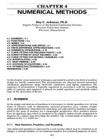
Figure
16.1
shows
a
cantilevered ring segment
fixed
at C. The
force
F
causes bend-
ing,

torsion,
and
direct shear.
The
moments
and
torques
at the
fixed
end C and at any
section
B are
shown
in
Table 16.3.
The
shear
at C is
R
c
= F.
Stresses
in the
ring
can be
computed using
the
formulas
of
Chap.

49.
To
obtain
the
deflection
at end
A,
we use
Castigliano's theorem. Neglecting
direct shear
and
noting
from
Fig.
16.16
that
/
= r
d0,
we
determine
the
strain energy
from
Table
16.2
to
be
pAPrd*
,

f*r
2
r<*9
^l
"2ET
+
J
0
"^F
(163)
Then
the
deflection
y at A and in the
direction
of F is
computed
from
>-f-;K«>*<sf№
The
terms
for
this relation
are
shown
in
Table
16.3.
It is
convenient

to
arrange
the
solution
in the
form
Fr
3
(A
B
\
,_
y
=
-T
(EI
+
GK)
(16
'
5)
where
the
coefficients
A and B are
related only
to the
span angle. These
are
listed

in
Table
16.3.
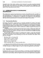
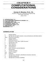
Figure
16.20
shows another cantilevered ring segment, loaded
now by a
dis-
tributed
load.
The
resultant load
is W =
wrfy
a
shear reaction
R = W
acts upward
at
the
fixed
end C, in
addition
to the
moment
and
torque
reactions shown
in
Table

16.3.
A
force
W=
wrQ
acts
at the
centroid
of
segment
AB in
Fig.
16.26.
The
centroidal
radius
is
?=
2rsini6/21
(166)
6
TABLE
16.1
Eccentricities
and
Stress Factors
for
Curved
Beams
1

1.
Rectangle
2.
Solid
round
3.
Hollow round
4.
Hollow rectangle
TABLE
16.1
Eccentricities
and
Stress Factors
for
Curved
Beams
1
(Continued)
5.
Trapezoid
6.
T
Section
fNotation:
r
»
radius
of
curvature

to
centroidal
axis
of
section;
A
»
area;
/
«
second moment
of
area;
e
«
distance
from
centroidal axis
to
neutral axis;
<r/
-
Kp
and
<T
O
-
Kjr
where
<r/

and
a
0
are the
normal stresses
on the
fibers
having
the
smallest
and
largest radii
of
curvature,
respectively,
and a are the
corresponding stresses computed
on
the
same
fibers
of a
straight beam. (Formulas
for
A and / can be
found
in
Table
48.1.)
7.

U
Section
TABLE
16.2
Strain
Energy
Formulas
Loading
Formula
1.
Axial
force
F
F*l
2AE
2.
Shear
force
F
rj
F*l
U
=
2AG
3.
Bending
moment
M
rj
m

f
M
2
<**
J
2EI
4.
Torsional
moment
T
1*1
2GK
To
determine
the
deflection
of end A, we
employ
a
fictitious
force
Q
acting down
at
end A.
Then
the
deflection
is
at/

r
f*
,,
9M
.
0
r
f*
3T
,
D
„,
_.
y
=
de
=
^i
M
3c
"
e+
^i
r
ae
"
e
(16J)
The
components

of the
moment
and
torque
due to Q can be
obtained
by
substitut-
ing
Q for
Fin
the
moment
and
torque equations
in
Table 16.3
for an end
load
F;
then
the
total
of the
moments
and
torques
is
obtained
by

adding this result
to the
equa-
tions
for M and T due
only
to the
distributed load. When
the
terms
in Eq.
(16.7) have
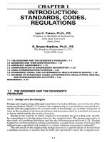
FIGURE 16.1
(a)
Ring segment
of
span angle
(J)
loaded
by
force
F
normal
to the
plane
of the
ring.
(b)
View
of

portion
of
ring
AB
showing positive
directions
of the
moment
and
torque
for
section
at B.
TABLE
16.3
Formulas
for
Ring
Segments
with
One
Support
Loading
Term
Formula
End
load
F
Moment
M-Fr

sin B
M
c
=
Fr sin
<f>
Torque
T
=
Fr(I
- cos
B)
T
c
*
Fr(I
- cos
</>)
dM
ST
Derivatives
—
=
r sin B —
=
K1
— cos 6)
or
dr
Deflection

A =
0
— sin
<f>
cos
0
coefficients
B
=
30
—
4 sin
0
+ sin
0
cos 0
Distributed
load
w;
fictitious
load
Q
Moment
M
=
Wr
2
O
- cos
0)

A/
c
-
wr\\
- cos
0)
Torque
T
=
wrfy
-
sin
6)
T
c
-
wr
2
^
-
sin
0)
^M
ar
Denvatives
—7:
=
r sin B
——
=

r(
1 — cos B)
d(2
oQ
Deflection
A
=
2 - 2 cos
4>
-
sin
2
0
coefficients
B
=
^
2
—
20
sin
0
+
sin
2
0
been
formed,
the
force

Q can be
placed equal
to
zero prior
to
integration.
The
deflection
equation
can
then
be
expressed
as
wr
4
(A
B
\
„,<>,
y=
-T
U
+
OT)
(16
'
8)
FIGURE 16.2
(a)

Ring segment
of
span angle
(J)
loaded
by a
uniformly
distributed load
w
acting
normal
to the
plane
of the
ring segment;
(b)
view
of
portion
of
ring
AB;
force
W is the
resultant
of the
distributed load
w
acting
on

portion
AB of
ring,
and it
acts
at the
centroid.
16.4
RINGSWITHSIMPLESUPPORTS
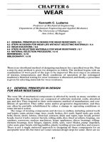
Consider
a
ring loaded
by any set of
forces
F and
supported
by
reactions
R, all
nor-
mal
to the ring
plane, such that
the
force system
is
statically determinate.
The
system
shown

in
Fig. 16.3, consisting
of
five
forces
and
three reactions,
is
statically determi-
nate
and is
such
a
system.
By
choosing
an
origin
at any
point
A on the
ring,
all
forces
and
reactions
can be
located
by the
angles

$
measured counterclockwise
from
A. By
treating
the
reactions
as
negative forces,
Den
Hartog
[16.3],
pp.
319-323,
describes
a
simple method
of
determining
the
shear force,
the
bending moment,
and the
tor-
sional moment
at any
point
on the ring. The
method

is
called
Biezeno's
theorem.
A
term called
the
reduced
load
P is
defined
for
this method.
The
reduced load
is
obtained
by
multiplying
the
actual load, plus
or
minus,
by the
fraction
of the
circle
corresponding
to its
location

from
A.
Thus
for a
force
F
h
the
reduced load
is
P^F
1
(16-9)
Then
Biezeno's
theorem states that
the
shear force
V
A
,
the
moment
M
4
,
and the
torque
T
A

at
section
A, all
statically indeterminate,
are
found
from
the set of
equations
V^=SP,
n
M
A
=
^
P
1
Y
sin to
(16.10)
n
T
A
=
^
P
1
T(I
-
COS

to)
n
where
n =
number
of
forces
and
reactions together.
The
proof uses Castigliano's the-
orem
and may be
found
in
Ref.
[16.3].
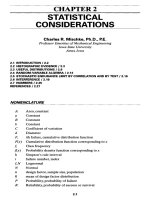
FIGURE
16.3 Ring loaded
by a
series
of
concentrated forces.
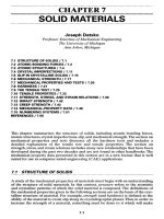
Example
1.
Find
the
shear force, bending moment,
and
torsional moment

at the
location
of
.R
3
for the
ring shown
in
Fig. 16.4.
Solution.
Using
the
principles
of
statics,
we
first find
the
reactions
to be
R
1
=
R
2
=
R
3
=
^F

Choosing
point
A at
R
3
,
the
reduced loads
are
p
$r
R
-o
P-ljf-o.o^
—H«.=-ilt™-
P,
=
||F=0.5833F
'-I* !!'-^"
Then, using
Eq.
(16.10),
we
find
V
A
=
O.
Next,
M

A
=
^
Fjrsin^
5
-
Fr
(O
+
0.0833
sin 30° -
0.2222
sin
120°
+
0.5833
sin
210°
_
0.4444
sin
240°)
=
-0.0576Fr
In a
similar manner,
we
find
T
A

=
0.991Fr.
FIGURE
16.4 Ring loaded
by the two
forces
F and
sup-
ported
by
reactions
RI,
R
2
,
and
R
3
.
The
crosses indicate
that
the
forces
act
downward;
the
heavy dots
at the
reac-

tions
R
indicate
an
upward direction.
The
task
of
finding
the
deflection
at any
point
on a
ring with
a
loading like that
of
Fig. 16.3
is
indeed
difficult.
The
problem
can be set up
using
Eq.
(16.2),
but the
result-

ing
integrals
will
be
lengthy.
The
chances
of
making
an
error
in
signs
or in
terms dur-
ing
any of the
simplification processes
are
very great.
If a
computer
or
even
a
programmable calculator
is
available,
the
integration

can be
performed using
a
numerical
procedure such
as
Simpson's rule (see Chap.
4).
Most
of the
user's manu-
als
for
programmable calculators contain such programs
in the
master library. When
this
approach
is
taken,
the two
terms behind each integral should
not be
multiplied
out or
simplified; reserve these tasks
for the
computer.
16.4.1
A

Ring
with
Symmetrical
Loads
A
ring having three equally spaced loads,
all
equal
in
magnitude, with three equally
spaced
supports located midway between each pair
of
loads,
has
reactions
at
each
support
of
R =
F/2,
M =
0.289Fr,
and T =
O
by
Biezeno's theorem.
To
find

the
moment
and
torque
at any
location
0
from
a
reaction,
we
construct
the
diagram shown
in
Fig.
16.5. Then
the
moment
and
torque
at A are
M
=
M
1
cos
9
-
R

1
T
sin 0
(16.11)
-
Fr
(0.289
cos
0 -
0.5
sin 0)
T=
M
1
sin 0 -
R
1
T
(I
- cos 0)
(16.12)
=
Fr
(0.289
sin 0 - 0.5 + 0.5 cos 0)
FIGURE 16.5
The
positive directions
of the
moment

and
torque axes
are
arbi-
trary.
Note that
^
1
=
F/2
and
M
1
=
0.289Fr.
MOMENT
AXIS
TORQUE
AXIS'
Neglecting direct shear,
the
strain energy stored
in the
ring between
any two
sup-
ports
is,
from
Table 16.2,

"->№<^
Castigliano's theorem states that
the
deflection
at the
load
F is
-f=i/>f-^r^f*
vw
From
Eqs.
(16.11)
and
(16.12),
we
find
-^
=
r(0.289cos0-0.5sin0)
or
rlT
^-
=
r(0.289
sin 0 - 0.5 + 0.5 cos 0)
or
When
these
are
substituted into

Eq.
(16.14),
we get
Fr
3
(A
B
\
/,ric\
y
=
-Y(EJ
+
GK)
(1615)
which
is the
same
as Eq.
(16.5).
The
constants
are
/-7E/3
A =
4
J
(0.289
cos 0 - 0.5 sin
0)

2
dQ
(16.16)
c
n/3
V
'
B
=
4
\
(0.289
sin 0 - 0.5 + 0.5 cos
0)
2
d0
J
o
These equations
can be
integrated directly
or by a
computer using Simpson's rule.
If
your
integration
is
rusty,
use the
computer.

The
results
are A =
0.1208
and B =
0.0134.
16.4.2
Distributed Loading
The
ring segment
in
Fig. 16.6
is
subjected
to a
distributed load
w
per
unit circumfer-
ence
and is
supported
by the
vertical reactions
#1
and
R
2
and the
moment reactions

MI
and
M
2
.
The
zero-torque reactions mean that
the
ring
is
free
to
turn
at A and B.
The
resultant
of the
distributed load
is W =
wr§;
it
acts
at the
centroid:
_
=
2TSiTlMi
<l>
By
symmetry,

the
force reactions
are
RI
=
R
2
=
W
12
-
wr§!2.
Summing moments
about
an
axis through
BO
gives
IM(BO)
=
-M
2
+
Wr
sin
|-
-
M
1
cos

(n
-
<|>)
-
^-
sin
$
=
O
Since
M
1
and
M
2
are
equal, this equation
can be
solved
to
give
FIGURE 16.6 Section
of
ring
of
span angle
$
with distributed
load.
M

1
=
WtI
1
-"**-***
2
)**+]
(16-18)
L
1 -
COS
(J)
J
Example
2. A
ring
has a
uniformly distributed load
and is
supported
by
three
equally
spaced reactions. Find
the
deflection midway between supports.
Solution.
If we
place
a

load
Q
midway between supports
and
compute
the
strain energy using
half
the
span,
Eq.
(16.7)
becomes
W 2r
(
¥2
,
_
3M
,_
2r
[^
2
„
3T
^
,_
im
y
=

^=TiI
M
-*Q
dQ+
GKl
T
tQ
dQ
(1619)
Using
Eq.
(16.18)
with
ty =
271/3
gives
the
moment
at a
support
due
only
to
w
to be
MI
=
0.395
wr
2

.
Then, using
a
procedure quite similar
to
that used
to
write Eqs.
(16.11)
and
(16.12),
we
find
the
moment
and
torque
due
only
to the
distributed load
at any
section
0 to be
M
w
=
wr
2
M

-
0.605
cos 0 -
^
sin 0
J
(16.20)
T
w
=
wr
2
1G
-
0.605
sin
0 - - +
^
cos
0
j
In a
similar manner,
the
force
Q
results
in
additional components
of

MQ
=
Qj-
(0.866
cos 0 - sin 0)
(16.21)
T
Q
=
&-
(0.866
sin 0 - 1 + cos 0)
3M
Q
r
Then
~T—
=
—
(0.866
cos 0 - sin 0)
o(2
2
/^)
1
T
-—f-
=
-£-
(0.866

sin
9
- 1 + cos
6)
oQ
2
And so,
placing
the
fictitious
force
Q
equal
to
zero,
Eq.
(16.19) becomes
y
=
^-\
(1
-
0.605
cos
0 -
^
sin
0
]
(0.866

cos
0 -
sin
0)
d0
EI
J
o
\
3
/
+
7^7
f
(
e
-
°-
605
sin
e
~
T
+
T
cos
6
J
(°-
866

sin
0 - 1 +
cos
0)
d0
(16.22)
GK
J
o
\
33/
When
this expression
is
integrated,
we
find
^(of-lf)
2
\ Ll
LrK
/
16.5
RINGSEGMENTSWITHFIXEDENDS
A
ring segment with
fixed
ends
has a
moment reaction

MI,
a
torque reaction
Ti
9
and
a
shear reaction
7?i,
as
shown
in
Fig.
16.7«.
The
system
is
indeterminate,
and so all
three relations
of Eq.
(16.2) must
be
used
to
determine them, using zero
for
each
corresponding displacement.
16.5.1

Segment
with
Concentrated
Load
The
moment
and
torque
at any
position
0 are
found
from
Fig.
16.76
as
M
=
TI
sin 0 +
M
1
cos 0 -
R^r
sin 0 +
Fr
sin (0 - y)
T
=
-T

1
cos 0 +
MI
sin 0 -
#ir(l
- cos 0) +
Fr[I
- cos (0 -
y)]
These
can be
simplified;
the
result
is
M
=
T
1
sin 0 +
M
1
cos 0 -
R
1
T
sin 0 + Fr cos y sin 0 - Fr sin y cos 0
(16.24)
T=
-Ti

cos 0 +
M
1
sin 0 -
/V(I
- cos 0)
-Fr
cos y cos 0 - Fr sin y sin 0 + Fr
(16.25)
Using
Eq.
(16.3)
and the
third relation
of Eq.
(16.2) gives
^-i?f«£**<5?f
r
£-»-»
<'«
6
>
Note
that
^-
=
cos0
oMi
dT
.

Q
^T-T
=
SIn
0
9M
1
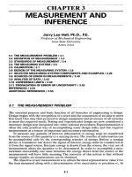
FIGURE 16.7
(a)
Ring segment
of
span angle
(|)
loaded
by
force
E (b)
Portion
of
ring used
to
com-
pute moment
and
torque
at
position
6.
Now
multiply

Eq.
(16.26)
by EI and
divide
by
r;
then substitute.
The
result
can be
written
in the
form
/4
(T
1
sin
9
+
MI
cos
9
-
R
1
T
sin
9)
cos
9

dQ
J
o
+
Fr J
(cos
y
sin 0 - sin
y
cos 9) cos 9
dQ
Y
EI
fr*
+
——
]
[-7\
cos 0 +
MI
sin 9 -
R^(I
- cos
0)]
sin 0
dQ
GK
l/o
f
*

1
-
Fr
(cos
Y
cos 0 + sin
Y
sin 0 - 1) sin 0
dQ
[ =
O
(16.27)
T
J
Similar
equations
can be
written using
the
other
two
relations
in Eq.
(16.2). When
these three relations
are
integrated,
the
results
can be

expressed
in the
form
a
n
«i
2
«13
T
1
IFr
^
1
«21
a
22
«23
M
1
IFr
=
b
2
(16.28)
a
31
a
32
0
33

J
[R
1
IF
J
\b
3
_
where
«11
=
sin
2
(J) ^
sin
2
^)
(16.29)
LrK
«21
=
(<!>-
sin
<|>
cos
(|>)
+
——
($
+ sin ty cos

<|>)
(16.30)
GK
EI
«31
=
(0
- sin
(()
cos
$)
+
——
((()
+ sin
§
cos
<|)
- 2 sin
(())
(16.31)
GK
EI
«12
=
(<!>
+ sin
(|)
cos
(|>)

+
——
((])
- sin
(|)
cos
(|>)
(16.32)
GA.
«
22
=
«n
(16.33)
~FI
«32
=
sin
2
0
+
-^-
[2(1
- cos
<|>)
-
sin
2
<|)]
(16.34)

GK
«13
=
~«32
(16.35)
«23
=
-«31
(16.36)
EI
«33
=
-(<|>
- sin
(|)
cos
<|>)
-
——
(3(|)
- 4 sin
$
+ sin ty cos
(|>)
(16.37)
GA
EI
b
1
= sin

Y
sin ty cos
((>
- cos
Y
sin
2
$
+
(0
-
Y)
sin
Y+
7^77
[cos
Y
sin
2
ty
GK
- sin
Y
sin fy cos
<|)
+
(<|)
-
Y)sin
Y

+ 2 cos ty - 2 cos
Y]
(16.38)
b
2
=
(Y-(^)
cos
Y~
sin
Y+
cos
Ysin
<|>
cos
<|>
+ sin
Ysin
2
0
£7
+
——
[(Y
-
(|>)
cos
Y
- sin
Y

+ 2 sin ty - cos
Y
sin
(|)
cos ty - sin
Y
sin
2
c|>]
(16.39)
GA
£
3
= (y-
(|>)
cos Y- sin
Y+
cos
Ysin
ty cos
(|)
+ sin
Ysin
2
ty
+
[(Y-
(|>)
cos
Y~

sin Y- cos
Ysin
ty cos ty - sin
Ysin
2
<|)
GK
+
2(sin
(|)
-
(|)
+
Y
+ cos
Y
sin
(|)
- sin
Y
cos
$)]
(16.40)
For
tabulation purposes,
we
indicate these relations
in the
form
FT FT

a
'i
=
Xi
i
+
Hk
Yii
bk
=
Xk+
GK
Yk
(16
'
41)
Programs
for
solving equations such
as Eq.
(16.28)
are
widely available
and
easy
to
use. Tables 16.4
and
16.5 list
the

values
of the
coefficients
for a
variety
of
span
and
load angles.
TABLE
16.4
Coefficients
a
tj
for
Various Span Angles
Span angle
</>
Coefficients
3r/2
*
3w/4
2*/3
w/2
ir/3
*/4
an
X
11
1 O 0.5

0.75 0.75
0.5
Y
1
I
-1 O
-0.5 -0.75
-
-0.75 -0.5
a
2
i
X
2
i
4.7124
TT
2.8562 2.5274 .5708 0.6142 0.2854
F
2
i
4.7124
TT
1.8562 1.6614 .5708 1.4802 1.2854
A
31
JT
31
4.7124
TT

2.8562 2.5274 .5708 0.6142 0.2854
Y
31
6.7124
T
0.4420
-0.0707 -0.4292 -0.2518 -0.1288
a
n
X
12
4.7124
T
1.8562 1.6614 .5708 1.4802 1.2854
Y
12
4.7124
T
2.8562 2.5274 .5708 0.6142 0.2854
a
22
X
22
I
O 0.5
0.75 0.75
0.5
Y
22
-1 O

-0.5 -0.75
-
-0.75 -0.5
a
32
X
32
1 O 0.5
0.75 0.75
0.5
K
32
1 4
2.9142
2.25 0.25
0.0858
a
n
X
13
-1 O
-0.5 -0.75
-
-0.75 -0.5
Y
13
-I
-4
-2.9142
-2.25

-
-0.25
-0.0858
«23
X
23
-4.7124
-»
-2.8562 -2.5274 -1.5708 -0.6142 -0.2854
X
23
-6.7124
-TT
-0.4420
0.0707
0.4292 0.2518 0.1288
a
33
X
33
-4.7124
-TT
-2.8562 -2.5274 -1.5708 -0.6142 -0.2854
K
33
-18.1372
-ST
-3.7402
-2.3861
-0.7124 -0.1105 -0.0277

TABLE
16.5
Coefficients
b
k
for
Various
Span
Angles
(J)
and
Load
Angles
y in
Terms
of ty
Coefficients,
Span
angle
0
load
angles
I I I
I
I
7
37T/2
TT
37T/4
27T/3

7T/2
7T/3
7T/4
,
X
1
2.8826 1.6661
0.2883
-0.0806 -0.4730 -0.4091 -0.2780
0>
Y
1
2.8826
-1.7481 -1.4019
1.0806
-0.4730 -0.1162 -0.0396
-
h
X
2
-1.3525
-2.3732 -2.1628
-1.8603
-1.0884 -0.4051 -0.1849
4
2
Y
2
-5.2003 -2.3732 -0.4727 -0.1283
0.1462

0.1022
0.0535
,
X
3
-1.3525 -2.3732 -2.1628 -1.8603 -1.0884 -0.4051 -0.1849
^
3
Y
3
-13.0342
-5.6714 -2.0455
-1.2699
-0.3622 -0.0544 -0.0135
h
X
1
3.1416
1.8138
0.4036
0.0446
-0.3424 -0.3179
-0.2180
1
r,
3.1416
-1.1862 -1.0106 -0.7817 -0.3424 -0.0839 -0.0286
^
,
X

2
O
-1.9132 -1.8178 -1.5620 -0.9069 -0.3346 -0.1522
3
°
2
Y
2
-4
-1.9132 -0.4036 -0.1307
0.0931
0.0706
0.0373
,X
3
O
-1.9132 -1.8178 -1.5620 -0.9069 -0.3346 -0.1522
b
*
Y
3
-10.2832
-4.3700 -1.5452 -0.9536 -0.2692 -0.0401
-0.0099
h
X
1
2.3732
1.5708
0.4351

0.1569
-0.1517 -0.1712 -0.1203
1
Y
1
2.3732
-0.4292 -0.4379 -0.3431 -0.1517 -0.0372 -0.0127
^
X
2
1.6661
-1
-1.1041 -0.9566 -0.5554 -0.2034 -0.0922
2
b
2
Y
2
-1.7481
-1
-0.2311 -0.0906
0.0304
0.0286
0.0154
,
X
3
1.6661
-1
-1.1041 -0.9566 -0.5554 -0.2034 -0.0922

°*
Y
3
-5.0463 -2.1416 -0.7395 -0.4529 -0.1262 -0.0186
-0.0046
16.5.2
Deflection
Due to
Concentrated
Load
The
deflection
of a
ring segment
at a
concentrated load
can be
obtained using
the
first
relation
of Eq.
(16.2).
The
complete analytical solution
is
quite lengthy,
and so a
result
is

shown here that
can be
solved using computer solutions
of
Simpson's
approximation. First, define
the
three solutions
to Eq.
(16.28)
as
T
1
=
C
1
Fr
M
1
=
C
2
Fr
R
1
=
C
3
F
(16.42)

Then
Eq.
(16.2)
will
have
four
integrals, which
are
o
A
F
=
[(C
1
-
C
3
)
sin
G
+
C
2
cos
6]
2
dQ
(16.43)
J
o

BF=
\
(cos
y sin 0 - sin y
cos
9)
2
dQ
(16.44)
J
o
C
F
=
\
[(C
3
-
C
1
)
cos
0
+
C
2
sin
9
-
C

3
]
2
dQ
(16.45)
J
o
D
F
=I
[I-
(cos
Y
cos
9
+ sin
y
sin
9)]
2
dB
(16.46)
•'o
The
results
of
these
four
integrations should
be

substituted into
y=
^r[
AF+BF+
~GK
(CF+DF)
]
(16
-
47)
to
obtain
the
deflection
due to F and at the
location
of the
force
E
It is
worth noting that
the
point
of
maximum deflection will never
be
far
from
the
middle

of the
ring, even though
the
force
F may be
exerted near
one
end.
This means
that
Eq.
(16.47)
will
not
give
the
maximum deflection unless
y=
(|>/2.
16.5.3
Segment
with
Distributed
Load
The
resultant load acting
at the
centroid
B'
in

Fig. 16.8
is
W=
wrc|),
and the
radius
r
is
given
by Eq.
(16.6), with
(|)
substituted
for 9.
Thus
the
shear reaction
at the
fixed
end
A is
.R
1
=
wr([)/2.
M
1
and
T
1

,
at the
fixed
ends,
can be
determined using Castigliano's
method.
We
use
Fig. 16.9
to
write equations
for
moment
and
torque
for any
section, such
as
the one at D.
When
Eq.
(16.6)
for r is
used,
the
results
are
found
to be

M
=
T
1
sin 0 +
M
1
cos
9
-
^-
sin
9 +
wr^l
-
cos
9)
(16.48)
T=
-T
1
cos 9 +
M
1
sin 9 -
^^-
(1 - cos 9) +
wr
2
(9

- sin 9)
(16.49)
FIGURE 16.8 Ring segment
of
span angle
(J)
subjected
to a
uniformly dis-
tributed load
w
per
unit circumference acting downward. Point
B'
is the
centroid
of
the
load.
The
ends
are
fixed
to
resist bending moment
and
torsional moment.
FIGURE 16.9
A
portion

of the
ring
has
been
isolated
here
to
determine
the
moment
and
torque
at any
section
D at
angle
6
from
the
fixed
end at A.
These equations
are now
employed
in the
same manner
as in
Sec.
16.5.1
to

obtain
h
Hf
s^i=tei
(
i6
-
5
°)
L«21
<*22
J
[M
1
1
1
WT
2
I
\b
2
\
It
turns
out
that
the
a^
terms
in the

array
are
identical with
the
same
coefficients
in
Eq.
(16.28); they
are
given
by
Eqs. (16.29), (16.30), (16.32),
and
(16.33), respectively.
The
coefficients
b
k
are
b
k
=
X
k
+
-^Y
k
(16.51)
CrA

where
X
1
=
^-
sin
2
ty + sin
(|>
cos
<|)
+
§
- 2 sin
§
(16.52)
YI
=
(j)
- 2 sin
<|)
-
-^-
sin
2
<|)
- sin
§
cos ty +
§(l

+ cos
(|))
(16.53)
TABLE
16.6
Coefficients
b
k
for
Various Span Angles
and
Uniform Loading
Span angle
</>
Coefficients
3ir/2
TT
3ir/4
2v/3
v/2
*/3
*/4
,
X
}
9.0686 3.1416 1.0310 0.7147 0.3562 0.1409 0.0675
D{
Y
1
9.0686 3.1416 1.5430 1.0572 0.3562 0.0602 0.0156

,
X
2
10.1033 0.9348 0.4507 0.3967 0.2337 0.0716 0.0263
°
2
Y
2
8.1033 0.9348
-1.7274 -2.0102 -1.7663
-0.9750
-0.5810
X
2
=
^ 2(1-
cos
(|>)
-
-|
sin
<|>
cos
(|>
+
sin
2
<|>
(16.54)
Y

2
=
-^-
- 2(1 - cos
(|>)
+
^-
sin
(|>
cos
<|>
-
sin
2
<|>
+
<|>
sin
<|>
(16.55)
Solutions
to
these equations
for a
variety
of
span angles
are
given
in

Table 16.6.
A
solution
for the
deflection
at any
point
can be
obtained using
a
fictitious load
Q at any
point
and
proceeding
in a
manner similar
to
other developments
in
this
chapter.
It is,
however,
a
very lengthy analysis.
REFERENCES
16.1 Raymond
J.
Roark

and
Warren
C.
Young, Formulas
for
Stress
and
Strain,
6th
ed.,
McGraw-Hill,
New
York,
1984.
16.2 Joseph
E.
Shigley
and
Charles
R.
Mischke, Mechanical Engineering Design,
5th
ed.,
McGraw-Hill,
New
York,
1989.
16.3
J. P. Den
Hartog, Advanced Strength

of
Materials,
McGraw-Hill,
New
York,
1952.