Sổ tay tiêu chuẩn thiết kế máy P48 docx

CHAPTER
41
LINKAGES
Richard
E.
Gustavson
Technical
Staff
Member
The
Charles
Stark Draper
Laboratory,
Inc.
Cambridge,
Massachusetts
41.1 BASIC LINKAGE
CONCEPTS/41.1
41.2 MOBILITY CRITERION
/
41.4
41.3
ESTABLISHING PRECISION POSITIONS
/
41.4
41.4 PLANE FOUR-BAR LINKAGE
/
41.4
41.5
PLANE OFFSET SLIDER-CRANK LINKAGE
/

41.8
41.6
KINEMATIC ANALYSIS
OF THE
PLANAR FOUR-BAR LINKAGE
/
41.8
41.7
DIMENSIONAL
SYNTHESIS
OF THE
PLANAR FOUR-BAR LINKAGE:
MOTION
GENERATION/41.10
41.8 DIMENSIONAL SYNTHESIS
OF THE
PLANAR FOUR-BAR LINKAGE: CRANK-
ANGLE COORDINATION
/41.18
41.9 POLE-FORCE
METHOD/41.20
41.10 SPATIAL
LINKAGES/41.21
REFERENCES/41.22
Linkages
are
mechanical devices that appear very straightforward
to
both ana-
lyze

and
design. Given proper technique, that
is
generally
the
case.
The
methods
described
in
this chapter reveal
the
complexity (and,
I
think,
the
beauty)
of
linkages.
I
have gained significant satisfaction during
my 20
years
of
work with them
from
both theoretical
and
functioning hardware standpoints.
47.7

BASICLINKAGECONCEPTS
41.1.1
Kinematic Elements
A
linkage
is
composed
of
rigid-body members,
or
links,
connected
to one
another
by
rigid
kinematic elements,
or
pairs.
The
nature
of
those connections
as
well
as the
shape
of the
links determines
the

kinematic properties
of the
linkage.
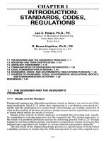
Although many kinematic pairs
are
conceivable
and
most
do
physically exist,
only
four
have general practical
use for
linkages.
In
Fig.
41.1,
the
four
cases
are
seen
to
include
two
with
1
degree
of

freedom
(/=
1), one
with
/= 2, and one
with
/= 3.
Single-degree-of-freedom
pairs constitute joints
in
planar linkages
or
spatial link-
ages.
The
cylindrical
and
spherical joints
are
useful
only
in
spatial linkages.
The
links which connect these kinematic pairs
are
usually binary (two connec-
tions)
but may be
tertiary (three connections)

or
even more.
A
commonly used ter-
tiary
link
is the
bell
crank familiar
to
most machine designers. Since
our
primary
FIGURE 41.1 Kinematic
pairs
useful
in
linkage design.
The
quantity
/
denotes
the
number
of
degrees
of
freedom.
interest
in

most linkages
is to
provide
a
particular output
for a
prescribed input,
we
deal
with
closed kinematic chains, examples
of
which
are
depicted
in
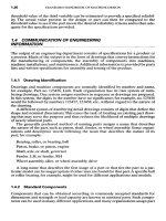
Fig. 41.2. Con-
siderable work
is now
under
way on
robotics, which
are
basically open chains (see
Chap. 47).
Here
we
restrict ourselves
to the
closed-loop type. Note that many com-

plex
linkages
can be
created
by
compounding
the
simple four-bar linkage. This
may
not
always
be
necessary once
the
design concepts
of
this chapter
are
applied.
41.1.2
Freedom
of
Motion
The
degree
of
freedom
for a
mechanism
is

expressed
by the
formula
F=M/-;-l)
+
£/,
(41.1)
i
= 1
FIGURE
41.2 Closed kinematic
chains,
(a)
Planar
four-bar
linkage;
(b)
planar six-bar
linkage;
(c)
spherical
four-bar
linkage;
(d)
spatial RCCR four-bar linkage.
where
/ =
number
of
links

(fixed
link included)
j
=
number
of
joints
ft
= /of
/th
joint
K
=
integer
=
3 for
plane, spherical,
or
particular spatial linkages
=
6 for
most spatial linkages
Since
the
majority
of
linkages used
in
machines
are

planar,
the
particular case
for
plane mechanisms with
one
degree
of
freedom
is
found
to be
2/-3/
+ 4
=
0
(41.2)
Thus,
in a
four-bar linkage, there
are
four
joints (either
re
volute
or
prismatic).
For a
six-bar
linkage,

we
need seven such joints.
A
peculiar special case occurs when
a
suf-
ficient
number
of
links
in a
plane linkage
are
parallel, which leads
to
such special
devices
as the
pantograph.
Considerable theory
has
evolved over
the
years about numerous aspects
of
link-
ages.
It is
often
of

little help
in
creating usable designs. Among
the
best references
available
are
Hartenberg
and
Denavit
[41.9],
Hall
[41.8],
Beyer
[41.1],
Hain
[41.7],
Rosenauer
and
Willis
[41.10],
Shigley
and
Uicker
[41.11],
and Tao
[41.12].
41.1.3
Number Synthesis
Before

you can
dimensionally synthesize
a
linkage,
you may
need
to use
number
synthesis,
which establishes
the
number
of
links
and the
number
of
joints that
are
required
to
obtain
the
necessary mobility.
An
excellent description
of
this subject
appears
in

Hartenberg
and
Denavit
[41.9].
The
four-bar linkage
is
emphasized here
because
of its
wide applicability.
47.2
MOBILITYCRITERION
In any
given four-bar linkage, selection
of any
link
to be the
crank
may
result
in its
inability
to
fully
rotate. This
is not
always necessary
in
practical mechanisms.

A
cri-
terion
for
determining whether
any
link might
be
able
to
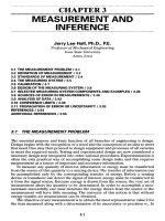
rotate 360° exists. Refer
to
Fig.
41.3, where
/,
s,
p,
and q are
defined.
Grubler's
criterion states that
l
+
s<p
+ q
(41.3)
If
the
criterion
is not

satisfied, only double-rocker linkages
are
possible. When
it is
satisfied,
choice
of the
shortest link
as
driver will result
in a
crank-rocker linkage;
choice
of any of the
other three links
as
driver will result
in a
drag link
or a
double-
rocker mechanism.
A
significant
majority
of the
mechanisms that
I
have designed
in

industry
are the
double-rocker type. Although they
do not
possess some theoretically desirable char-
acteristics, they
are
useful
for
various types
of
equipment.
41.3 ESTABLISHING PRECISION POSITIONS
In
designing
a
mechanism with
a
certain number
of
required precision positions,
you
will
be
faced with
the
problem
of how to
space them.
In

many practical situations,
there will
be no
choice, since particular conditions must
be
satisfied.
If
you do
have
a
choice, Chebychev spacing should
be
used
to
reduce
the
struc-
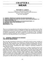
tural error. Figure 41.4 shows
how to
space
four
positions within
a
prescribed inter-
val
[41.9].
I
have found that
the
end-of-interval

points
can be
used instead
of
those
just
inside with good results.
47.4 PLANE
FOUR-BAR
LINKAGE
41.4.1
Basic
Parameters
The
apparently simple four-bar linkage
is
actually
an
incredibly sophisticated device
which
can
perform wonders once proper design techniques
are
known
and
used. Fig-
ure
41.5 shows
the
parameters required

to
define
the
general case. Such
a
linkage
can be
used
for
three types
of
motion:
1.
Crank-angle coordination Motion
of
driver link
b
causes prescribed motion
of
link
d.
2.
Path
generation Motion
of
driver link
b
causes point
C to
move along

a
pre-
scribed path.
3.
Motion generation Movement
of
driver link
b
causes line
CD to
move
in a
pre-
scribed planar motion.
FIGURE 41.3 Mobility
characteristics,
(a)
Closed
four-link
kinematic chain:
/ =
longest link,
s =
short-
est
link,/?,
q =
intermediate-length links;
(b)
crank rocker linkage;

(c)
double-rocker linkage.
FIGURE
41.4
Four-precision-point
spacing
(Chebychev)
XI=X
A
+
0№Sl(x
B
-
XA)
X
2
=
X
A
+
0.3087(*
5
-
X
A
)
x
3
=
x

A
+
0.6913(*
B
-
XA)
x
4
=
x
A
+
0.9619(*
B
-
X
A
)
In
general,
for n
precision
points
Xj
=
-(XA+XB)
\
(
x
7l(2/-l)

.
.
-
(XB-XA)COS
^
2n
*
;
=
l,2, ,n
41.4.2
Kinematic Inversion
A
very
useful
concept
in
mechanism design
is
that
by
inverting
the
motion,
new
interesting
characteristics
become
evident.
By

imagining yourself
attached
to
what
is
actually
a
moving body,
you can
determine various properties, such
as the
location
of
a
joint which connects that body
to its
neighbor. This technique
has
been found use-
ful
in
many industrial applications, such
as the
design
of the
four-bar automobile
window regulator
([41.6]).
41.4.3
Velocity Ratio

At
times
the
velocity
of the
output will need
to be
controlled
as
well
as the
corre-
sponding position. When
the
motion
of the
input crank
and the
output crank
is
coor-
dinated,
it is an
easy matter
to
establish
the
velocity ratio
co<//co
6

.
When
you
extend
line
AB in
Fig. 41.5 until
it
intersects
the
line through
the
fixed
pivots
O
A
and
O
B
in
a
point
S
9
you
find
that
^t
=
°£

(41
4)
co,
0
A
0
B
+
0
A
S
^
'
;
Finding
the
linear
velocity
of a
point
on the
coupler
is not
nearly
as
straightforward.
A
very
good
approximation

is to
determine
the
travel
distance
along
the
path
of the
point
during
a
particular
motion
of the
crank.
41.4.4 Torque Ratio
Because
of the
conservation
of
energy,
the
following
relationship
holds:
T
b
d$
=

T
d
dy
(41.5)
FIGURE
41.5 General
four-bar
linkage
in a
plane.
Since both sides
of
(41.5)
can be
divided
by dt, we
have,
after
some rearranging,
•-£-^-t
(4i
-
6
>
The
torque ratio
n is
thus
the
inverse

of the
velocity ratio. Quite
a few
mechanisms
that
I
have designed have made significant
use of
torque ratios.
41.4.5
Transmission
Angle
For the
four-bar linkage
of
Fig. 41.5,
the
transmission angle
T
occurs between
the
coupler
and the
driven link. This angle should
be as
close
to 90° as
possible. Useful
linkages
for

motion generation have been created with
T
approaching
20°.
When
a
crank rocker
is
being designed,
you
should
try to
keep
45° < T <
135°.
Double-rocker
or
drag link mechanisms usually have other criteria which
are
more significant than
the
transmission angle.
4
7.5
PLANE OFFSET
SLIDER-CRANK
LINKAGE
A
variation
of the

four-bar linkage which
is
often
seen occurs when
the
output link
becomes infinitely long
and the
path
of
point
B is a
straight line. Point
B
becomes
the
slider
of the
slider-crank linkage. Although coupler
b
could have
the
characteristics
shown
in
Fig. 41.6,
it is
seldom used
in
practice.

Here
we are
interested
in the
motion
of
point
B
while crank
a
rotates.
In
general,
the
path
of
point
B
does
not
pass
through
the
fixed
pivot
O
A
,
but is
offset

by
dimension
e. An
obvious example
of the
degenerate case
(E
=
O) is the
piston crank
in an
engine.
The
synthesis
of
this linkage
is
well described
by
Hartenberg
and
Denavit
[41.9].
I
have used
the
method many times
after
programming
it for the

digital computer.
41.6
KINEMATIC ANALYSIS
OF THE
PLANAR
FOUR-BARLINKAGE
41.6.1
Position Geometry
Refer
to
Fig. 41.7, where
the
parameters
are
defined. Given
the
link lengths
a,
b,
c,
and d and the
crank position angle
(|>,
the
angular position
of
coupler
c is
9
=

TC
- (T +
\|f)
(41.7)
FIGURE 41.6 General
offset
slider-crank linkage.
FIGURE
41.7 Parameters
for
analysis
of a
four-bar
linkage.
The
driven link
d
will
be at
angle
!
h
2
+
a
2
-b
2
l
h

2
+
d
2
-c
2
//n
0
,
V
=
C
°
S
—Wb~
+
C
°
S
-2W—
(4L8)
where
h
2
=
a
2
+
b
2

+
2abcosty
(41.9)
The
transmission angle
i
will
be
1
c
2
+
d
2
-a
2
-b
2
-
2ab cos
(|)
//M
1/v
.
T
=
cos-
1
—
*•

(41.10)
A
point
on
coupler
P has
coordinates
P
x
= -b cos
$
+
r
cos (0 + a)
J
P
y
=
Z?sin(|)
+
rsin(e
+
a)
(41.11)
41.6.2
Velocity
and
Acceleration
The
velocity

of the
point
on the
coupler
can be
expressed
as
dP
x
,
d<b
.
.
dQ
.
/tt
v
-T^
=
b
-f
1
sin
6 - r
——
sin
(9 + a)
dt
dt
^

dt
^
'
(41.12)
dP,
rf6
^e
/D
,
-T^-
=
Z?
-T
11
cos
d>
+ r — cos (0 + a)
dt
dt dt
^
'
As you can
see,
the
mathematics gets very complicated very rapidly.
If you
need
to
establish velocity
and

acceleration data, consult Ref.
[41.1],
[41.7],
or
[41.11].
Com-
puter analysis
is
based
on the
closed vector loop equations
of C. R.
Mischke, devel-
oped
at
Pratt Institute
in the
late 1950s.
See
[41.19], Chap.
4.
41.6.3
Dynamic
Behavior
Since
all
linkages have clearances
in the
joints
as

well
as
mass
for
each link, high-
speed operation
of a
four-bar linkage
can
cause very undesirable behavior. Methods
for
solving these problems
are
very complex.
If you
need
further
data, refer
to
numerous
theoretical articles originally presented
at the
American Society
of Me-
chanical
Engineers (ASME) mechanism conferences. Many have been published
in
ASME journals.
47.7
DIMENSIONALSYNTHESIS

OF
THE
PLANAR
FOUR-BAR
LINKAGE:
MOTION
GENERATION
41.7.1
Two
Positions
of a
Plane
The
line
A
1
B
1
defines
a
plane (Fig. 41.8) which
is to be the
coupler
of the
linkage
to
be
designed. When
two
positions

are
defined,
you can
determine
a
particular point,
called
the
pole
(in
this case
P
i2
,
since
the
motion goes
from
position
1 to
position
2).
The
significance
of the
pole
is
that
it is the
point about which

the
motion
of the
body
is
a
simple rotation;
the
pole
is
seen
to be the
intersection
of the
perpendicular bisec-
tors
OfAiA
2
and
BiB
2
.
A
four-bar linkage
can be
created
by
choosing
any
point

on
^
2
as
O
A
and any
reasonable point
on
bib
2
as
O
B
.
Note that
you do not
have
a
totally arbitrary choice
for
the
fixed
pivots, even
for
this elementary case. There
are
definite limitations,
since
the

four-bar linkage must produce continuous motion between
all
positions.
When
a
fully
rotating crank
is
sought,
the
Grubler criterion must
be
adhered
to. For
double-rocker mechanisms,
the
particular link lengths still have definite criteria
to
meet.
You
have
to
check these
for
every four-bar linkage that
you
design.
41.7.2
Three Positions
of a

Plane
When
three positions
of a
plane
are
specified
by the
location
of
line
CD, as
shown
in
Fig.
41.9,
it is
possible
to
construct
the
center
of a
circle through
Ci,
C
2
,
and
C

3
and
through
DI,
D
2
,
and
D
3
.
This
is
only
one of an
infinite combination
of
links that
can
be
attached
to the
moving body containing line
CD. If the
path
of one end of
line
CD
lies
on a

circle, then
the
other
end can
describe points
on a
coupler path which cor-
respond
to
particular rotation angles
of the
crank (Fig.
41.10);
that
is a
special case
of
the
motion generation problem.
The
general three-position situation describes three poles
Pi
2
,
Pi
3
,
and
P
23

which
form
a
pole
triangle.
You
will
find
this triangle
useful
since
its
interior angles
(6i
2
/2
in
Fig. 41.9) define precise geometric relationships between
the
fixed
and
moving piv-
ots of
links which
can be
attached
to the
moving body defined
by
line

CD.
Examples
of
this geometry
are
shown
in
Fig.
41.11,
where
you can see
that
FIGURE 41.8
Two
positions
of a
plane: definition
of
pole
P
n
.
S-PuPuPn
=
S-A
1
PuOA
=
^B
1

P
12
Oz
(41.13)
The
direction
in
which these angles
are
measured
is
critical.
For
three positions,
you
may
thus choose
the
fixed
or the
moving pivot
and use
this relationship
to
establish
the
location
of the
corresponding moving
or

fixed
pivot, since
it is
also
true that
S-PuPuP*
=
^A
1
P
13
O*
=
^B
1
P
13
O
8
(41.14)
The
intersection
of two
such lines (Fig.
41.12)
is the
required pivot point. Note that
the
lines defined
by the

pole triangle relationships extend
in
both directions
from
the
pole; thus
a
pivot-point angle
may
appear
to be
±180°
from
that defined within
the
triangle. This
is
perfectly valid.
It is
important
to
observe that arbitrary choices
for
pivot locations
are
available
when
three positions,
or
less,

of the
moving plane
are
specified.
FIGURE 41.9 Three positions
of a
plane: definition
of the
pole
tri-
angle
P
12
P
13
P
23
-
41.7.3
Four
Positions
of a
Moving
Plane
When
four
positions
are
required, appropriate pivot-point locations
are

precisely
defined
by
theories generated
by
Professor Burmester
in
Germany during
the
188Os.
His
work
[41.2]
is the
next step
in
using
the
poles
of
motion. When
you
define
four
positions
of a
moving plane containing line
CD as
shown
in

Fig.
41.13,
six
poles
are
defined:
PU
P\3
PU
P?2>
P^
P$4
By
selecting opposite poles
(P
n
,
P
34
and
P
13
,
P
24
),
you
obtain
a
quadrilateral with sig-

nificant
geometric relationships.
For
practical purposes, this opposite-pole quadrilat-
eral
is
best used
to
establish
a
locus
of
points which
are the
fixed
pivots
of
links that
can
be
attached
to the
moving body
so
that
it can
occupy
the
four
prescribed positions.

This
locus
is
known
as the
center-point
curve
(Fig.
41.14)
and can be
found
as
follows:
1.
Establish
the
perpendicular bisector
of the two
sides
Pi
2
P
2
4
and
Pi
3
P
34
.

2.
Determine points
M and
M'
such that
Z-Pi
2
MQ
2
=
^
Pi
3
M'Q
3
3.
With
M as
center
and
MPi
2
as
radius, create circle
k.
With
M'
as
center
and

M'Pi
3
as
radius, create circle
k''.
4. The
intersections
of
circles
k and
k'
(shown
as
C
0
and
CQ
in
Fig.
41.14)
are
center
points
with
the
particular property that
the
link whose
fixed
pivot

is
C
0
or
CQ
has a
FIGURE
41.10 Path
generation
as a
special
case
of
motion
generation,
total rotation angle twice
the
value defined
by the
angle(s)
in
step
2. The
magni-
tude
and
direction
of the
link angle
^

14
are
defined
in the
figure.
Note that this construction
can
produce two, one,
or no
intersection points. Thus
some link rotations
are not
possible. Depending
on how
many angles
you
want
to
investigate, there
will
still
be
plenty
of
choices.
I
have
found
it
most convenient

to
solve
the
necessary analytic geometry
and
program
it for the
digital computer;
as
many
accurate results
as
desired
are
easily determined.
Once
a
center point
has
been established,
the
corresponding moving pivot (circle
point)
can be
established.
For the
first
position
of the
moving body,

you
need
to use
the
pole triangle
Pi
2
PnP
23
angles
to
establish
two
lines whose intersection
will
be the
circle point.
In
Fig.
41.15,
the
particular angles
are
^Pi
3
Pi
2
P
23
^c

1
P
12
C
0
FIGURE
41.11 Geometric relationship between pole triangle angle(s)
and
location
of
link
fixed
and
moving pivot points.
and
360°
-
LP
23
P
13
P
12
=
^c
1
P
13
C
0

The
second equality could also
be
written
/.P
23
P
13
P
12
-
^c
1
P
13
C
0
+
180°
A
locus
of
points thus defined
can be
created
as
shown
in
Fig.
41.16.

Each point
on
the
circle-point curve corresponds
to a
particular point
on the
center-point curve.
Some possible links
are
defined
in
Fig.
41.16;
each
has a
known first-to-fourth-
position rotation angle. Only those links whose length and/or pivot locations
are
within
prescribed limits need
to be
retained.
The two
intermediate positions
of the
link
can be
determined
by

establishing
the
location
of the
moving pivot (circle point)
in the
second
and
third positions
of the
moving
body. Since
the
positions
lie on the arc
with center
at the
fixed
pivot (center
point)
a and
radius
aa\
it is
easy
to
determine
the
link rotation angles
as

(h
=
LA
1
OAA
2
(I)
13
-
LA
1
OAA
3
Linkages need
to be
actuated
or
driven
by one of the
links. Knowing
the
three
rotation angles allows
you to
choose
a
drive link which
has the
desired proportions
FIGURE 41.12 Determining

the
moving
or
fixed
pivot
by
using
the
pole triangle.
FIGURE
41.13 Four positions
of a
plane: definition
of the
opposite-pole quadrilateral formed
by
lines
P
13
P
24
and
P
n
P*.
FIGURE
41.14 Determination
of
points
on the

center-point curve.
FIGURE
41.15 Determination
of a
circle point corresponding
to a
particular center point.
FIGURE 41.16 Some
of the
links which
can be
attached
to the
plane containing
CD.
of
motion.
Proper
care
in
selection
of the two
links will result
in a
smooth-running
four-bar
linkage.
41.7.4
Five
Positions

of a
Plane
It
would seem desirable
to
establish
as
many precision positions
as
possible.
You can
choose
two
sets
of
four
positions (for example, 1235
and
1245)
from
which
the
Burmester curves
can be
created.
The
intersections
(up to
six)
of

those
two
center-
point curves
are the
only
fixed
pivots which
can be
used
to
guide
the
moving body
through
the
five
positions. Since those pivots and/or link lengths have virtually
always
been outside
the
prescribed limits,
I
never
use
five-position synthesis.
41.7.5
Available
Computer
Programs

Two
general-purpose planar linkage synthesis programs have been created: KIN-
SYN
([41.17])
and
LINCAGES
([41.18]).
They involve
the
fundamentals described
in
this section
and can be
valuable when time
is
limited.
I
have found
it
more advan-
tageous
to
create
my own
design
and
analysis programs, since
the
general programs
almost always need

to be
supplemented
by
routines that define
the
particular prob-
lem
at
hand.
47.8
DIMENSIONALSYNTHESIS
OF THE
PLANAR
FOUR-BAR
LINKAGE:
CRANK-ANGLE
COORDINATION
Many
mechanical movements
in
linkages depend
on the
angular position
of the
out-
put
crank.
In
general,
you

will have
to
design
the
four-bar linkage
so
that
a
pre-
scribed input crank rotation will produce
the
desired output crank rotation.
Significant
work
was
performed
in an
attempt
to
generate functions
([41.9])
using
the
four-bar linkage until
the
advent
of the
microcomputer. Although
it is
seldom

necessary
to
utilize
the
function
capability,
you
will
find
many applications
for
crank-angle
coordination.
Two
methods
are
possible: geometric
and
analytical.
41.8.1
Geometric Synthesis
In
a
manner similar
to
that
for
motion generation (Sec. 41.7),
the
concept

of the
pole
is
once again fundamental. Here, however,
it is a
relative
pole, since
it
defines rela-
tive
motions. Suppose that
you
need
to
coordinate
the
rotation angles
(J)
12
for the
crank
(input)
and
\|/
12
for the
follower (output). Refer
to
Fig.
41.17,

where
the
fol-
lowing
steps have been drawn:
1.
Establish convenient locations
for the
fixed
pivots
O
A
and
O
B
-
2.
Draw
an
extended
fixed
link
O
A
O
B
.
3.
With
OA

as
vertex,
set off a
line
€ at
angle
-c|>
12
/2
(half rotation angle,
opposite
direction).
FIGURE
41.17
Crank-angle
coordination:
definition
of
relative pole
Q
u
-
4.
With
OB
as
vertex,
set off a
line
€'

at
angle
-\j/i
2
/2
(half
rotation angle, opposite
direction).
5. The
intersection
of € and
€'
is the
relative pole
Qi
2
.
6.
Using
Qi
2
as the
vertex,
set off the
angle
Z-A
1
Q
12
B

1
=
^OAQ
12
O
8
in
any
convenient location, such
as
that shown.
When
only
two
positions
are
required,
you may
choose
A
1
and
B
1
anywhere
on
the
respective sides
of the
angle drawn

in
step
6. For
three positions,
two
relative
poles
Qi
2
and
Q
13
are
used.
You may
arbitrarily choose either
A
1
or
B
1
,
but the
other
pivot must
be
found
geometrically. Figure 41.18 shows
the
necessary constructions.

41.8.2
Analytical
Synthesis
Although
four-bar
linkages
had
been studied analytically
for
about
100
years,
it was
not
until 1953 that Ferdinand Freudenstein [41.4] derived
the now
classic relation-
ship
^
1
cos
<|>
-
R
2
cos
\j/
+
R
3

= cos
(c|)
-
\|/)
(41.15)
FIGURE
41.18
Geometric
construction
method
for
three
crank-angle
position
coordination.
where
a
R
_a
b
2
-c
2
+
d
2
+
a
2
^i

=
~7
^2-~r
*<3-
0
,
,
a
5
20d
These link lengths
are
described
in
Fig. 41.7. With
Eq.
(41.15)
you can
establish
a
sig-
nificant
variety
of
linkage requirements.
The
first
derivative
of the
Freudenstein

equation
is
(R
1
sin
+)
(f)
-
(R
2
sin
V
)
(^)
=
(f
-
^)
sin
(+
-
¥
)
(41.16)
which
provides
a
relationship
for the
velocity

or
torque
ratio.
By
using
the
relation-
ship
in
Sec. 41.4.4,
Eq.
(41.16) becomes
^
1
sin
c|>
-
nR
2
sin
x|f
= (1 -
n)
sin
(<|)
- Y)
(41.17)
where
n
is the

torque
or
velocity ratio.
A
further
derivative which would deal with
accelerations
has
never
been
useful
to me. If the
need arises,
see
Ref.
[41.9].
Since
the
problem
is one of
crank-angle coordination,
there
are
potentially
five
unknowns
(Ri
9
R
2

,
R
3
,
fa and
XJf
1
)
which
you
could determine. Combinations
of fa,
X|f
ly:
,
and
HJ
may be
specified such that
a
series
of
equations
of the
form
R
1
cos
((I)
1

+
(J)
17
-)
-
R
2
cos
(\|/!
+
x|f
ly
)
+
R
3
= cos
(^
1
+ fa
-XJf
1
-
xjf
ly
)
(41.18)
and
^
1

sin
((J)
1
+
<|>
1;
.)
- rty/?
2
sin
(XjI
1
+
X|/
1;
)
=
(1 -
n
}
)
sin
((J)
1
+
<|>
1;
.)
-XJf
1

-
xj/
ly
)
(41.19)
can
be set up and
solved.
The
nonlinear characteristic makes
the
solution compli-
cated. Results
for
certain cases
may be
found
in
[41.9]
and
[41.11].
I
have found
it
most
useful
in a
digital computer program
to
vary

fa
over
the
range
O to
n
in
four
simultaneous equations. This produces loci
for the
moving pivot-point
locations
which
go
through
the
relative poles
and are
reminiscent
of
Burmester curves.
The
two
sets
of
four
conditions likely
to be of
practical interest
are as

follows:
1.
Specify
crank rotations
(J)
12
,
(I)
1
S,
$14,
xj/
12
,
x|/
13
,
and
xj/
14
.
2.
Specify
crank rotations
and
velocity
or
torque
ratios
^

12
,
/I
1
,
XJf
12
,
and
n
2
.
41.9
POLE-FORCE
METHOD
An
extremely
useful
scheme
for
determining static balancing forces
in a
plane link-
age
was
developed
by
Hain [41.7]
and
popularized

by Tao
[41.12].
Although
it is
potentially
useful
for
design,
I
have used
it
primarily
to
analyze
the
requirements
for
counterbalance springs.
Statically
balancing
the
force
on the
coupler
of a
four-bar
linkage
is a
problem
often

encountered.
The
solution requires knowledge
of the
forces and/or torques
acting
on the
four-bar linkage
as
well
as
determination
of the
instantaneous centers.
Refer
to
Fig.
41.19«,
in
which
the
following
constructions occur:
1. The
intersection
T
1
of
forces
F

ab
and
F
ac
is
found.
2. The
intersection
of the
coupler (extended) with force
F
ab
is
S
ab
and
with
F
ac
is
S
ac
.
FIGURE 41.19 Pole-force
method
for
balancing
a
force
on the

coupler
of a
four-bar
linkage.
3.
Determine lines
S
ab
(ab)
and
S
ac
(ac);
their intersection
is
T
2
.
4.
Line
TiT
2
closes
the
pole-force triangle, which
is
transferred
to
Fig.
41.19Z?.

5. The
magnitude
of
F
ab
required
to
balance
the
coupler
force
F
ac
is
easily
found.
Many
other cases,
any of
which
you
might encounter
in
practice,
are
shown
by Tao
[41.12].
47.70
SPATIALLINKAGES

Most practical linkages have motion entirely
in a
plane
or
possibly
in two
parallel
planes with duplicated mechanisms such
as
those
in a
backhoe
or a
front
loader.
Design procedures
for
some elementary types
of
spatial four-bar linkage have been
created (Refs. [41.9]
and
[41.11]),
principally
for the
RGGR
type (Fig. 41.20).
Three principal mathematical methods
for
writing

the
loop-closure equation
are
vectors
([41.3]),
dual-number quaternions
([41.14]),
and
matrices
([41.13]).
These
techniques have evolved into general-purpose computer programs such
as IMP
FIGURE
41.20
An
RGGR
spatial
linkage;
R
designates
a
revolute
joint,
G
desig-
nates
a
spherical
joint.

([41.16])
and
ADAMS
and
DRAM
([41.5]);
they
will
make
your
spatial
linkage
anal-
ysis
much
easier.
With
such
tools
available,
you can
design
complex
spatial
mecha-
nisms
by
iterative
analysis.
REFERENCES

41.1 Rudolph
A.
Beyer, Kinematic
Synthesis
of
Mechanisms,
Herbert Kuenzel
(trans.),
McGraw-Hill,
New
York,
1964.
41.2
Ludwig Burmester, Lehrbuch
der
Kinematick
(in
German only),
A.
Felix, Leipzig,
1888.
41.3 Milton
A.
Chace, "Vector Analysis
of
Linkages,"
/.
Eng.
Ind.,
ser.

B,
vol.
55, no. 3,
August
1963,
pp.289-297.
41.4
Ferdinand Freudenstein, "Approximate Synthesis
of
Four-Bar Linkages,"
Trans.
ASME,
vol.
77, no.
6,1955,
pp.
853-861.
41.5 Ferdinand Freudenstein
and
George Sandor, "Kinematics
of
Mechanisms,"
in
Harold
A.
Rothbart (ed.),
Mechanical
Design
and
Systems

Handbook,
2d
ed.,
McGraw-Hill,
New
York,
1985.
41.6 Richard
E.
Gustavson,
"Computer-Designed
Car-Window
Linkage,"
Mech.
Eng.,
Septem-
ber
1967,
pp.
45-51.
41.7 Kurt Hain, Applied Kinematics,
2d
ed.,
Herbert Kuenzel,
T. P.
Goodman,
et
al.
(trans.),
McGraw-Hill,

New
York,
1967.
41.8 Allen
S.
Hall,
Jr.,
Kinematics
and
Linkage Design, Prentice-Hall, Englewood
Cliffs,
NJ.,
1961.
41.9
Richard
S.
Hartenberg
and
Jacques Denavit, Kinematic
Synthesis
of
Linkages,
McGraw-
Hill,
New
York,
1964.
41.10
N.
Rosenauer

and A. H.
Willis, Kinematics
of
Mechanisms,
Dover,
New
York,
1967.
41.11 Joseph
E.
Shigley
and
John
J.
Uicker,
Jr.,
Theory
of
Machines
and
Mechanisms,
McGraw-
Hill,
New
York,
1980.
41.12
D. C.
Tao, Applied Linkage
Synthesis,

Addison-Wesley,
Reading,
Mass.,
1964.
41.13 John
J.
Uicker,
Jr.,
J.
Denavit,
and R. S.
Hartenberg,
"An
Iterative Method
for the
Dis-
placement Analysis
of
Spatial Linkages,"
/
Appl.
Mech.,
vol.
31,
ASME
Trans.,
vol.
86,
ser.
E,

1964,
pp.
309-314.
41.14
An T.
Yang
and
Ferdinand Freudenstein, "Application
of
Dual-Number
and
Quaternion
Algebra
to the
Analysis
of
Spatial Mechanisms,"
/.
Appl
Mech. ASME
Trans.,
vol.
86,
ser.
E,
1964,
pp.
300-308.
41.15 ADAMS
and

DRAM, Automatic Dynamic Analysis
of
Mechanical
Systems
and
Dynamic
Response
of
Articulated
Machinery,
developed
by
Chace
at the
University
of
Michigan.
41.16
IMP,
the
Integrated
Mechanisms Program, developed
by
Uicker
at the
University
of
Wis-
consin.
41.17

KINSYN,
primarily
for
kinematic synthesis, developed
by
Kaufman while
at
M.I.T.
(he
is
now at
George Washington University).
41.18 LINCAGES,
for
kinematic synthesis
and
analysis, developed
by
Erdmann
et
al.
at the
University
of
Minnesota.
41.19
C R.
Mischke, Elements
of
Mechanical

Analysis,
Addison-Wesley,
Reading,
Mass.,
1963.