Sổ tay tiêu chuẩn thiết kế máy P57 pptx

CHAPTER
49
STRESS
Joseph
E.
Shigley
Professor
Emeritus
The
University
of
Michigan
Ann
Arbor,
Michigan
49.1
DEFINITIONS
AND
NOTATION
/
49.1
49.2 TRIAXIAL STRESS
/
49.3
49.3 STRESS-STRAIN RELATIONS
/
49.4
49.4
FLEXURE/49.10
49.5 STRESSES
DUE TO

TEMPERATURE
/49.14
49.6 CONTACT
STRESSES/49.17
REFERENCES
/
49.22
49.1
DEFINITIONS
AND
NOTATION
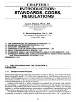
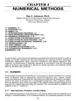
The
general two-dimensional stress element
in
Fig.
49.1«
shows
two
normal stresses
C
x
and
Gy,
both positive,
and two
shear stresses
i
xy
and
i

yx
,
positive also.
The
element
is
in
static equilibrium,
and
hence
i
xy
=
i
yx
.
The
stress state depicted
by the
figure
is
called plane
or
biaxial
stress.
FIGURE
49.1
Notation
for
two-dimensional

stress.
(From
Applied
Mechanics
of
Materials,
by
Joseph
E.
Shigley. Copyright
©
1976
by
McGraw-Hill,
Inc.
Used
with
permission
of the
McGraw-Hill
Book
Company.}
Figure
49.1b
shows
an
element
face
whose normal makes
an

angle
ty to the x
axis.
It can be
shown that
the
stress components
a and T
acting
on
this
face
are
given
by
the
equations
o
=
G^+G,
+
O
1
-O
2
,
CQS
^
+
^

^
n
^
(49
A)
T
= -
x
y
sin
2<|>
+
Tj
0
,
cos
2<|>
(49.2)
It can be
shown that when
the
angle
$
is
varied
in Eq.
(49.1),
the
normal stress
a has

two
extreme values. These
are
called
the
principal
stresses,
and
they
are
given
by the
equation
G,
+
G
V
17
G
x
-GyV
7
1
1/2
CT
1
,
G
2
=

-^
2
-
±
[(^y^j
+
4J
(49.3)
The
corresponding values
of fy are
called
the
principal directions.
These
directions
can
be
obtained
from
2(I)
=
IaIT
1
2lxy
(49.4)
O
x
-Gy
The

shear stresses
are
always zero when
the
element
is
aligned
in the
principal direc-
tions.
It
also turns
out
that
the
shear stress
T in Eq.
(49.2)
has two
extreme values. These
and the
angles
at
which they occur
may be
found
from
M=±
[(^)'
+

,.,]"
(49
,>
2$
=
tan'
1
-
a
*
"
°
y
(49.6)
^txy
The two
normal stresses
are
equal when
the
element
is
aligned
in the
directions
given
by Eq.
(49.6).
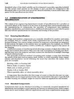
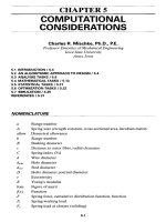
The act of
referring stress components

to
another
reference system
is
called
transformation
of
stress.
Such transformations
are
easier
to
visualize,
and to
solve,
using
a
Mohr's
circle
diagram.
In
Fig. 49.2
we
create
a
GT
coordinate system with nor-
mal
stresses plotted
as the

ordinates.
On the
abscissa, tensile (positive) normal
stresses
are
plotted
to the
right
of the
origin
O, and
compression (negative) normal
stresses
are
plotted
to the
left.
The
sign convention
for
shear
stresses
is
that clock-
wise
(cw) shear stresses
are
plotted above
the
abscissa

and
counterclockwise (ccw)
shear
stresses
are
plotted
below.
The
stress state
of
Fig.
49.Ia
is
shown
on the
diagram
in
Fig. 49.2. Points
A and C
represent
G
x
and
G
y
,
respectively,
and
point
E is

midway between them. Distance
AB
is
i
xy
and
distance
CD is
i
yx
.
The
circle
of
radius
ED
is
Mohr's
circle.
This circle passes
through
the
principal stresses
at F and G and
through
the
extremes
of the
shear
stresses

at H and /. It is
important
to
observe that
an
extreme
of the
shear stress
may
not
be the
same
as the
maximum.
FIGURE 49.2 Mohr's circle diagram
for
plane
stress.
(From
Applied Mechanics
of
Materials,
by
Joseph
E.
Shigley.
Copyright
©
7976
by

McGraw-Hill,
Inc.
Used
with permission
of the
McGraw-
Hill
Book
Company.)
49.1.1
Programming
To
program
a
Mohr's circle solution, plan
on
using
a
rectangular-to-polar
conversion
subroutine.
Now
notice,
in
Fig. 49.2, that
(a*
-
G
y
)/2

is the
base
of a
right triangle,
i
xy
is
the
ordinate,
and the
hypotenuse
is an
extreme
of the
shear stress. Thus
the
con-
version
routine
can be
used
to
output both
the
angle
2(|)
and the
extreme value
of the
shear stress.

As
shown
in
Fig. 49.2,
the
principal stresses
are
found
by
adding
and
subtracting
the
extreme value
of the
shear stress
to and
from
the
term
(G
X
+
G
y
)/2.
It is
wise
to
ensure,

in
your programming, that
the
angle
$
indicates
the
angle from
the x
axis
to
the
direction
of the
stress component
of
interest; generally,
the
angle
(()
is
considered
positive
when measured
in the ccw
direction.
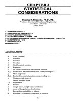
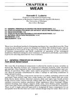
49.2
TRIAXIALSTRESS
The
general three-dimensional stress element

in
Fig.
49.30
has
three normal stresses
O
x
,
<3
y
,
and
G
V
all
shown
as
positive,
and six
shear-stress components, also shown
as
positive.
The
element
is in
static equilibrium,
and
hence
FIGURE 49.3
(a)

General
triaxial stress element;
(b)
Mohr's
circles
for
triaxial stress.
T — T T — T T — T
^xy
^yx
^yz
*zy
^zx
^xz
Note that
the
first
subscript
is the
coordinate normal
to the
element
face,
and the
second subscript designates
the
axis
parallel
to the
shear-stress component.

The
neg-
ative
faces
of the
element
will
have shear stresses acting
in the
opposite direction;
these
are
also considered
as
positive.
As
shown
in
Fig.
49.3b,
there
are
three principal stresses
for
triaxial stress states.
These three
are
obtained
from
a

solution
of the
equation
O
3
-
(G
x
+
a
y
+
G
Z
)0
2
+
(O
x
Cy
+
G
x
Oz
+
OyGz
-
T^
-
T£

-
T^)O
-
(G
x
GyOz
+
2vc
yz
T«
-
o/c£
-
o/c£
-
a,4)
-
O
(49.7)
In
plotting Mohr's circles
for
triaxial stress, arrange
the
principal stresses
in the
order
Oi
>
O

2
>
O
3
,
as in
Fig.
49.3£.
It can be
shown that
the
stress coordinates
OT
for
any
arbitrarily located plane
will
always
lie on or
inside
the
largest circle
or on or
outside
the two
smaller circles.
The
figure
shows that
the

maximum shear stress
is
always
W
=
^p
(49.8)
when
the
normal stresses
are
arranged
so
that
Oi
>
O
2
>
O
3
.
49.3
STRESS-STRAINRELATIONS
The
stresses
due to
loading described
as
pure

tension,
pure
compression,
and
pure
shear
are
o
=
f
T
=
f
(49.9)
where
F is
positive
for
tension
and
negative
for
compression
and the
word pure
means
that there
are no
other complicating
effects.

In
each case
the
stress
is
assumed
to be
uniform, which requires that
• The
member
is
straight
and of a
homogeneous material.
• The
line
of
action
of the
force
is
through
the
centroid
of the
section.
•
There
is no
discontinuity

or
change
in
cross section near
the
stress element.
• In the
case
of
compression,
there
is no
possibility
of
buckling.
Unit
engineering strain
e,
often
called simply unit
strain,
is the
elongation
or
deformation
of a
member subjected
to
pure axial loading
per

unit
of
original length.
Thus
e
=
-f
(49.10)
/o
where
8 =
total strain
/o
=
unstressed
or
original length
Shear
strain
y is the
change
in a
right angle
of a
stress element
due to
pure shear.
Hooke's
law
states that, within certain limits,

the
stress
in a
material
is
propor-
tional
to the
strain which produced
it.
Materials which regain their original shape
and
dimensions when
a
load
is
removed
are
called
elastic
materials.
Hooke's
law is
expressed
in
equation
form
as
a
=

£e
T-Gy
(49.11)
where
E = the
modulus
of
elasticity
and G = the
modulus
of
ridigity,
also called
the
shear
modulus
of
elasticity.
Poisson demonstrated that, within
the
range
of
Hooke's
law,
a
member subjected
to
uniaxial loading exhibits both
an
axial strain

and a
lateral strain. These
are
related
to
each other
by the
equation
lateral strain
v-
—
r-
(49.12)
axial
strain
where
v is
called Poisson's
ratio.
The
three constants given
by
Eqs.
(49.11)
and
(49.12)
are
often
called
elastic

con-
stants.
They have
the
relationship
E
=
2G(l+v)
(49.13)
By
combining Eqs. (49.9), (49.10),
and
(49.11),
it is
easy
to
show that
5
=
-§
(49.14)
which
gives
the
total deformation
of a
member subjected
to
axial tension
or

com-
pression.
A
solid round
bar
subjected
to a
pure twisting moment
or
torsion
has a
shear
stress that
is
zero
at the
center
and
maximum
at the
surface.
The
appropriate equa-
tions
are
t
=
-y-
V«
=

-y
(49.15)
where
T =
torque
p
=
radius
to
stress element
r
=
radius
of bar
/
=
second moment
of
area (polar)
The
total angle
of
twist
of
such
a
bar,
in
radians,
is

9
=
f
(49.16)
where
/ =
length
of the
bar.
For the
shear stress
and
angle
of
twist
of
other cross sec-
tions,
see
Table
49.1.
49.3.1
Principal
Unit
Strains
For a bar in
uniaxial tension
or
compression,
the

principal strains
are
ei
=
-?r
^
2
=-Ve
1
63 Ve
1
(49.17)
LL
Notice that
the
stress state
is
uniaxial,
but the
strains
are
triaxial.
For
triaxial stress,
the
principal
strains
are
G
1

VG
2
VCJ
3
ei
~~E~~E~~~E~
€2=
02_voi__vo3_
(4918)
LL
tL
tli
_
O
3
vai
vq
2
^~~E~~E~~E
These equations
can be
solved
for the
principal stresses;
the
results
are
Ee
1
(I

- v) +
v£(e
2
+
€
3
)
Gl
-
l-v-2v
2
_
Ee
2
(I-V)
+
VE(C
1
+
e
3
)
(49
19)
^-
l_v-2v
2
Ee
3
(I-V)+

V^(C
1
+
€
2
)
°3-
i_
v
_2v
2
The
biaxial stress-strain relations
can
easily
be
obtained
from
Eqs.
(49.18)
and
(49.19)
by
equating
one of the
principal stresses
to
zero.
TABLE
49.1 Torsional Stress

and
Angular Deflection
of
Various
Sections
t
Sectional shape Shape
constant
Shear
stress
1.
Solid round
2.
Round tube
3.
Square
[49.1]
TABLE
49.1
Torsional
Stress
and
Angular
Deflection
of
Various
Sectionsf
(Continued)
K=
t

(h-
O
3
~
T
~
2t(h
-
t)
2
K
=
~f
r
=
7T3A
+
1.8/Q
^-
3
+
1.462
^2.976
(^-
0.238
(^
_
2f(fr
-
/)

2
(/z
-
o
2
r
^
+
^-
2
^
TS
2/(^-/x/i-0
4.
Square tube, generous
fillets
[49.2]
I
5.
Rectangle [49.1]
6.
Rectangular tube, generous
fillets
[49.2]
Sectional shape
Shape
constant Shear
stress
7.
Hexagon

[49.1]
t
Deflection
is
O
=
Tl/KG
in
rad,
where
T =
torque,
/
=
length,
K =
shape constant,
and G =
modulus
of
rigidity.
See
[49.2]
for
additional shapes
in
torsion.
49.3.2
Plastic
Strain

It is
important
to
observe that
all the
preceding relations
are
valid only when
the
material obeys
Hooke's
law.
Some materials (see Sec. 7.9), when stressed
in the
plastic region, exhibit
a
behav-
ior
quite similar
to
that given
by Eq.
(49.11).
For
these materials,
the
appropriate
equation
is
a

=
#£"
(49.20)
where
a =
true stress
K
=
strength
coefficient
e =
true plastic strain
n =
strain-strengthening exponent
The
relations
for the
true stress
and
true strain
are
G
=
^-
E
=
UIy-
(49.21)
AI
IQ

where
A
1
and
//
are, respectively,
the
instantaneous values
of the
area
and
length
of a
bar
subjected
to a
load
F
1
.
Note that
the
areas
in
Eqs. (49.9)
are the
original
or
unstressed areas;
the

subscript zero
was
omitted,
as is
customary.
The
relations
between true
and
engineering (nominal) stresses
and
strains
are
o
= a exp e e =
ln(e
+1)
(49.22)
49.4
FLEXURE
Figure
49.4«
shows
a
member loaded
in
flexure
by a
number
of

forces
F and
sup-
ported
by
reactions
R
1
and
R
2
at the
ends.
At
point
C a
distance
x
from
R
1
,
we can
write
IMc =
2M
ext
+
M-O
(49.23)

where
ZM
ext
=
-xRi
+
C
1
Fi
+
C
2
F
2
and is
called
the
external
moment
at
section
C The
term
M,
called
the
internal
or
resisting
moment,

is
shown
in its
positive direction
in
both parts
b and c of
Fig. 49.4. Figure 49.5 shows that
a
positive moment causes
the
top
surface
of a
beam
to be
concave.
A
negative moment causes
the top
surface
to be
convex
with
one or
both ends curved downward.
A
similar relation
can be
defined

for
shear
at
section
C:
EFy
=
LF
6
Xt+
V=
O
(49.24)
where
LF
ext
=
R
1
-
F
1
-
F
2
and is
called
the
external
shear

force
at C. The
term
V,
called
the
internal
shear
force,
is
shown
in its
positive direction
in
both parts
b and c
of
Fig. 49.4.
Figure 49.6 illustrates
an
application
of
these relations
to
obtain
a set of
shear
and
moment diagrams.
FIGURE 49.4 Shear

and
moment.
(From
Applied Mechanics
of
Materials,
by
Joseph
E.
Shigley.
Copyright
©
1976
by
McGraw-Hill, Inc.
Used
with permission
of
the
McGraw-Hill
Book
Company.)
FIGURE 49.5 Sign conventions
for
bending.
(From
Applied
Mechan-
ics of
Materials,

by
Joseph
E.
Shigley.
Copyright
©
1976
by
McGraw-Hill,
Inc. Used
with permission
of
the
McGraw-Hill
Book
Company.)
POSITIVE
BENDING
FIGURE
49.6
(a)
View showing
how
ends
are
secured;
(b)
loading
diagram;
(c)

shear-force
dia-
gram;
(d)
bending-moment diagram. (From
Applied
Mechanics
of
Materials,
by
Joseph
E.
Shigley.
Copyright
©
1976
by
McGraw-Hill,
Inc.
Used
with permission
of
the
McGraw-Hill
Book
Company.)
The
previous relations
can be
expressed

in a
more general form
as
"-"
<«*>
If
the
flexure
is
caused
by a
distributed load,
dV
(J
1
M
/>|n
_.
—
=
-—-
=-w
(49.26)
dx
dx
2
where
w = a
downward-acting load
in

units
of
force
per
unit length.
A
more general
load distribution
can be
expressed
as
r
AF
q=hm
——
^
A*
->
o
Ax
where
q is
called
the
load
intensity;
thus
q = -w in Eq.
(49.26).
Two

useful
facts
can
be
learned
by
integrating Eqs. (49.25)
and
(49.26).
The
first
is
r
dV
=
r
qdx
=
V
B
-V
A
(49.27)
J
v
A
J
XA
which
states that

the
area
under
the
loading function between
X
A
and
X
B
is the
same
as
the
change
in the
shear
force
from
A to B.
Also,
f
B
dM=\
B
Vdx =
M
B
-M
A

(49.28)
V
4
J
*A
which
states that
the
area
of
the
shear-force
diagram between
X
A
and
X
B
is the
same
as
the
change
in
moment
from
A to B.
FIGURE 49.7
The
meaning

of the
term neutral
axis.
Note
the
difference
between
the
neutral axis
of
the
section
and the
neutral axis
of
the
beam.
(From
Applied
Mechanics
of
Materials,
by
Joseph
E.
Shigley.
Copyright
©
7976
by

McGraw-Hill,
Inc.
Used
with permission
of
the
McGraw-Hill
Book
Company.)
The
flexural
formula
is
O
1
=-^j-
(49.29)
for
the
section
of
Fig. 49.7.
The
formula states that
a
normal compression stress
o*
occurs
on a
fiber

at a
distance
y
from
the
neutral axis when
a
positive moment
M is
applied.
In Eq.
(49.29),
7
is the
second moment
of
area.
A
number
of
formulas
are
listed
in
Chap.
48.
The
maximum flexural stress occurs
at
y

max
= c at the
outer surface
of the
beam.
This
stress
is
often
written
in the
three forms
Mc
M M
/^om
0=
—
°
=
JTc
°
=
^
(4930)
Figure 49.7 distinguishes between
the
neutral
axis
of
a

section
and the
neutral
axis
of
a
beam,
both
of
which
are
often
referred
to
simply
as the
neutral
axis.
The
assump-
tions used
in
deriving
flexural
relations
are
• The
material
is
isotropic

and
homogeneous.
• The
member
is
straight.
• The
material obeys
Hooke's
law.
• The
cross section
is
constant along
the
length
of the
member.
•
There
is an
axis
of
symmetry
in the
plane
of
bending (see Fig. 49.7).
•
During pure bending (zero shear force), plane cross sections remain plane.

PLANE
OF
SYMMETRY
AND
PLANE
OF
BENDING
NEUTRAL AXIS
OF
BEAM
NEUTRAL
AXIS
OF
SECTION
where
Z is
called
the
section modulus. Equations (49.30)
can
also
be
used
for
beams
having
unsymmetrical sections provided that
the
plane
of

bending coincides with
one of the two
principal axes
of the
section.
When shear forces
are
present,
as in
Fig.
49.6c,
a
member
in flexure
will also
experience shear stresses
as
given
by the
equation
t-f-
(49.31)
where
b =
section width,
and Q =
first
moment
of a
vertical

face
about
the
neutral
axis
and is
Q
=
\ y
dA
(49.32)
y\
For a
rectangular section,
Q
=
fydA
=
bfydy
=
^(c
l
-yl)
>i
y\
£
Substituting
this value
of Q
into

Eq.
(49.31) gives
*
=
^(c
2
-yi)
Using
/
=
Ac
2
I?),
we
learn that
-IK)
The
value
of b for
other sections
is
measured
as
shown
in
Fig. 49.8.
In
determining shear stress
in a
beam,

the
dimension
b is not
always measured
parallel
to the
neutral axis.
The
beam sections shown
in
Fig. 49.8 show
how to
mea-
sure
b in
order
to
compute
the
static moment
Q. It is the
tendency
of the
shaded area
to
slide relative
to the
unshaded area which causes
the
shear stress.

Shear
flow
q is
defined
by the
equation
q
=
^j-
(49.34)
where
q is in
force units
per
unit length
of the
beam
at the
section under considera-
tion.
So
shear
flow is
simply
the
shear force
per
unit length
at the
section defined

by
y
=
yi.
When
the
shear
flow is
known,
the
shear stress
is
determined
by the
equation
T
=-J
(49.35)
49.5
STRESSESDUETOTEMPERATURE
A
thermal
stress
is
caused
by the
existence
of a
temperature gradient
in a

member.
A
temperature
stress
is
created
in a
member when
it is
constrained
so as to
prevent
expansion
or
contraction
due to
temperature change.
FIGURE
49.8
Correct
way to
measure
dimension
b to
determine
shear
stress
for
various
sections.

(From
Applied
Mechanics
of
Materials,
by
Joseph
E.
Shigley. Copyright
©
7976
by
McGraw-Hill, Inc.
Used
with
permission
of the
McGraw-Hill
Book
Company.}
49.5.1
Temperature
Stresses
These stresses
are
found
by
assuming that
the
member

is not
constrained
and
then
computing
the
stresses required
to
cause
it to
assume
its
original dimensions.
If the
temperature
of an
unrestrained member
is
uniformly
increased,
the
member
expands
and the
normal strain
is
e
x
=
t

y
=
€z
=
(X(AjT)
(49.36)
where
AT
=
temperature change
and a
=
coefficient
of
linear
expansion.
The
coeffi-
cient
of
linear expansion increases
to
some extent with temperature. Some mean
values
for
various materials
are
shown
in
Table 49.2.

Figure
49.9 illustrates
two
examples
of
temperature stresses.
For the bar in
Fig.
49.9«,
o*
=
-Oc(AT)E
G
y
=
o
z
=
-vo*
(49.37)
The
stresses
in the
flat
plate
of
Fig.
49.9b
are
a

x
=
c
y
=
-
0
^
_
o,
=
-vo*
(49.38)
TABLE
49.2
Coefficients
of
Linear Expansion
Celsius
scale Fahrenheit scale
Material
10
6
«
0
C
10
6
«
0

F
Aluminum
24.0
20-100
13.4 68-212
Aluminum
26.7
20-300
14.9
68-572
Brass
(cast) 18.75 0-100 10.4 32-212
Brass
(wire) 19.3 0-100 10.7 32-212
Brass
(spring) 19.8
25-300
11.0 77-572
Cast
iron 10.6
40 5.9 104
Carbon steel 10.8
40 6.0 104
Carbon steel
11.5
100-200
6.4
212-392
Carbon steel
15

300-400
8.3
572-752
Magnesium
(cast) 27.0
20-100
15.0 68-212
Nickel
steel (10%) 13.0
20 7.2 68
Stainless steel (hardened)
9.6
20-100
5.3
68-212
Stainless steel (hardened)
9.8
20-200
5.5
68-392
Stainless steel (annealed) 10.3
20-100
5.7
68-212
Stainless steel (annealed) 10.7
20-200
6.0
68-392
49.5.2
Thermal

Stresses
Heating
of the top
surface
of the
restrained
member
in
Fig.
49.1Oa
causes
end
moments
of
M
=
^P
(49.39)
and
maximum
bending
stresses
of
o,
=
±
^P
(49
.
40)

with
compression
of the top
surface.
If the
constraints
are
removed,
the bar
will
curve
to a
radius
FIGURE
49.9
Examples
of
temperature stresses.
In
each case
the
temperature rise
AT
is
uni-
form
throughout,
(a)
Straight
bar

with
ends restrained;
(b)
flat
plate
with
edges restrained.
FIGURE
49.10
Examples
of
thermal
stresses,
(a)
Rectangular member
with
ends restrained
(temperature
difference
between
top and
bottom results
in end
moments
and
bending stresses);
(b)
thick-walled
tube
has

maximum stresses
in
tangential
and
longitudinal directions.
h
"~
Ct(AT)
The
thick-walled
tube
of
Fig.
49.
Wb
with
a hot
interior surface
has
tangential
and
longitudinal
stresses
in the
outer
and
inner surfaces
of
magnitude
a(Ar>£

I"
2IfInWr,)]
°"
=
a
»
=
2(l-v)ln(r>,.)
i
1
-
rl-rl
\
(49
'
41)
-(X(AT)E
[
2r
0
2
ln(r
0
/n)l
,.„ ,
°"
=
^2(1-V)InU)
L
1

-^TT
1
J
(49
'
42)
where
the
subscripts
/
and o
refer
to the
inner
and
outer radii, respectively,
and the
subscripts
t and /
refer
to the
tangential (circumferential)
and
longitudinal direc-
tions. Radial stresses
of
lesser magnitude will also exist, although
not at the
inner
or

outer surfaces.
If
the
tubing
of
Fig.
49.10£
is
thin, then
the
inner
and
outer stresses
are
equal,
although
opposite,
and are
q(A7)£
°"
=
a
'°
=
2(1^0
(49.43)
Ct(AT)E
°"
=
°"

=
-2(1^0
at
points
not too
close
to the
tube ends.
49.6
CONTACTSTRESSES
When
two
elastic bodies having curved surfaces
are
pressed
against each other,
the
initial point
or
line
of
contact changes into area contact, because
of the
deformation,
and a
three-dimensional state
of
stress
is
induced

in
both bodies.
The
shape
of the
contact area
was
originally deduced
by
Hertz,
who
assumed that
the
curvature
of the
two
bodies could
be
approximated
by
second-degree surfaces.
For
such bodies,
the
contact area
was
found
to be an
ellipse. Reference [49.3] contains
a

comprehensive
bibliography.
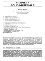
As
indicated
in
Fig.
49.11,
there
are
four
special cases
in
which
the
contact
area
is
a
circle.
For
these
four
cases,
the
maximum pressure occurs
at the
center
of the
con-
tact area

and is
p
Sf
(49
-
44)
where
a = the
radius
of the
contact area
and F = the
normal force pressing
the two
bodies together.
In
Fig.
49.11,
the x and y
axes
are in the
plane
of the
contact area
and the z
axis
is
normal
to
this plane.

The
maximum stresses occur
on
this axis, they
are
principal
stresses,
and
their values
for all
four
cases
in
Fig. 49.11
are
FIGURE
49.11 Contacting bodies having
a
circular contact
area,
(a) Two
spheres;
(b)
sphere
and
plate;
(c)
sphere
and
spherical socket;

(d)
crossed cylinders
of
equal
diameters.
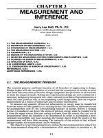
DISTANCE
BELOW
CONTACT SURFACE
FIGURE 49.12 Magnitude
of the
stress components
on the z
axis below
the
surface
as a
func-
tion
of the
maximum pressure. Note that
the two
shear-stress components
are
maximum
slightly
below
the
surface.
The
chart

is
based
on a
Poisson's
ratio
of
0.30.
The
radii
a of the
contact circles depend
on the
geometry
of the
contacting bod-
ies.
For two
spheres, each having
the
same diameter
d,
or for two
crossed cylinders,
each having
the
diameter
d, and in
each case with like materials,
the
radius

is
/3Fd
l-v
2
\
1/3
-(
1
TV-)
(49
'
47)
where
v and E are the
elastic constants.
For two
spheres
of
unlike materials having diameters
di
and
d
2
,
the
radius
is
a
=
[3F^_/

i
-v
i
+
i
-vi^
Ls
d
1
+d
2
\
E
1
E
2
;j
^
'
^=A(
i

a
^^
(i+v)
-w^\
(49
-
45)
"•-life

(49
-
46)
These equations
are
plotted
in
Fig. 49.12 together with
the two
shear stresses
i
xz
and
i
yv
Note that
i
xy
=
O
because
a*
=
a
r
RATIO
OF
STRESS
TO
P

0
For a
sphere
of
diameter
d and a
flat
plate
of
unlike materials,
the
radius
is
[W-W
For a
sphere
of
diameter
di
and a
spherical socket
of
diameter
d
2
of
unlike mate-
rials,
the
radius

is
"[far(^W
Contacting cylinders with parallel axes subjected
to a
normal force have
a
rect-
angular
contact area.
We
specify
an xy
plane coincident with
the
contact area with
the x
axis parallel
to the
cylinder axes. Then, using
a
right-handed coordinate system,
the
stresses along
the z
axis
are
maximum
and are
K
7

2
\
1/2
Zl
I
+
^)
-j\
(49.51)
K
l W
z
2
\
m
2zl
2
-T7Iw)(
1+
^)
—J
<
49
'
52)
^
(TrS^
(49
-
53)

where
the
maximum pressure occurs
at the
origin
of the
coordinate system
in the
contact zone
and is
2F
P
0
=
-^
(49.54)
where
/ = the
length
of the
contact zone measured parallel
to the
cylinder axes,
and
b = the
half
width. Equations (49.51)
to
(49.53) give
the

principal stresses. These
equations
are
plotted
in
Fig.
49.13.
The
corresponding shear stresses
can be
found
from
a
Mohr's circle; they
are
plotted
in
Fig.
49.14. Note that
the
maximum
is
either
i
xz
or
i
yz
depending
on the

depth below
the
contact
surface.
The
half width
b
depends
on the
geometry
of the
contacting cylinders.
The
fol-
lowing
cases arise most
frequently:
Two
cylinders
of
equal diameter
and of the
same
material have
a
half
width
of
"(^
1

TT
For two
cylinders
of
unequal diameter
and
unlike materials,
the
half width
is
^^(^+W
2
<
49
-
56
)
L
1C/
d
l
+
d
2
\
E
1
E
2
J]

DISTANCE BELOW CONTACT SURFACE
FIGURE 49.13 Magnitude
of the
principal stresses
on the z
axis below
the
surface
as a
func-
tion
of the
maximum pressure
for
contacting cylinders. Based
on a
Poisson's
ratio
of
0.30.
DISTANCE
BELOW
CONTACT SURFACE
FIGURE 49.14 Magnitude
of the
three shear stresses computed
from
Fig.
49.13.
RATIO

OF
STRESS
TO
P
0
RATIO
OF
STRESS
TO
P
Q
For a
cylinder
of
diameter
d in
contact with
a flat
plate
of
unlike material,
the
result
is
'-[¥(^W
The
half width
for a
cylinder
of

diameter
J
1
pressing against
a
cylindrical socket
of
diameter
J
2
of
unlike
material
is
^T^ri^^lT
<
49
-
58
>
L
TC/
d
2
-d
l
\
E
1
E

2
J]
REFERENCES
49.1
F. R.
Shanley, Strength
of
Materials,
McGraw-Hill,
New
York, 1957,
p.
509.
49.2
W. C.
Young, Roark's Formulas
for
Stress
and
Strain,
6th
ed., McGraw-Hill, 1989,
p.
348-359.
49.3
J. L.
Lubkin, "Contact Problems,"
in W.
Flugge
(ed.),

Handbook
of
Engineering Mechan-
ics,
McGraw-Hill,
New
York, 1962,
pp.
42-10
to
42-12.