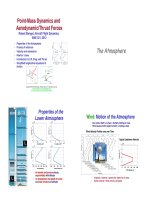
Aircraft Flight Dynamics Robert F. Stengel Lecture13 Analysis of Time Response

Time Response of Linear,
Time-Invariant Systems


Robert Stengel, Aircraft Flight Dynamics

MAE 331, 2012"
•  Time-domain analysis"
–  Transient response to initial conditions and
inputs"
–  Steady-state (equilibrium) response"
–  Continuous- and discrete-time models"
–  Phase-plane plots"
–  Response to sinusoidal input"
Copyright 2012 by Robert Stengel. All rights reserved. For educational use only.!
/>!
/>!
Linear, Time-Invariant (LTI)
Longitudinal Model"

Δ

V (t)
Δ

γ
(t)
Δ

q(t)
Δ

α

(t)
$
%
&
&
&
&
&
'
(
)
)
)
)
)
=
−D
V
−g −D
q
−D
α
L
V
V
N
0
L
q
V

N
L
α
V
N
M
V
0 M
q
M
α
−
L
V
V
N
0 1 −
L
α
V
N
$
%
&
&
&
&
&
&
&

&
'
(
)
)
)
)
)
)
)
)
ΔV(t)
Δ
γ
(t)
Δq(t)
Δ
α
(t)
$
%
&
&
&
&
&
'
(
)
)

)
)
)
+
0 T
δ
T
0
0 0 L
δ
F
/ V
N
M
δ
E
0 0
0 0 −L
δ
F
/ V
N
$
%
&
&
&
&
&
'

(
)
)
)
)
)
Δ
δ
E(t)
Δ
δ
T (t )
Δ
δ
F(t)
$
%
&
&
&
'
(
)
)
)
•  Steady, level flight"
•  Simplified control effects "
•  Neglect disturbance effects
"
•  What can we do with it?"

–  Integrate equations to obtain time histories of initial condition, control, and
disturbance effects"
–  Determine modes of motion"
–  Examine steady-state conditions"
–  Identify effects of parameter variations"
–  Define frequency response
"
Gain insights about
system dynamics!
Linear, Time-Invariant
System Model"
•  General model contains"
–  Dynamic equation (ordinary differential equation)"
–  Output equation (algebraic transformation) "
€
Δ
˙
x (t) = FΔx(t) + GΔu(t) + LΔw(t), Δx(t
o
) given
Δy(t) = H
x
Δx(t) + H
u
Δu(t) + H
w
Δw(t)
•  State and output dimensions need not be the same"
dim Δx(t )
[ ]

= n × 1
( )
dim Δy(t )
[ ]
= r × 1
( )
System Response to Inputs
and Initial Conditions"
•  Solution of the linear, time-invariant (LTI) dynamic model "

Δ

x(t) = FΔx(t) + GΔu(t) + LΔw(t), Δx(t
o
) given
Δx(t) = Δx(t
o
) + FΔx(
τ
) + GΔu(
τ
) + LΔw(
τ
)
[ ]
t
o
t
∫
d

τ
•  has two parts"
–  Unforced (homogeneous) response to initial conditions"
–  Forced response to control and disturbance inputs"
Response to
Initial Conditions
Unforced Response to
Initial Conditions"
•  The state transition matrix, Φ, propagates the
state from t
o
to t by a single multiplication"
Δx(t ) = Δx(t
o
)+ FΔx(
τ
)
[ ]
d
τ
t
o
t
∫
= e
F t−t
o
( )
Δx(t
o

) = Φ t − t
o
( )
Δx(t
o
)
e
F t −t
o
( )
= Matrix Exponential
= I + F t − t
o
( )
+
1
2!
F t − t
o
( )
"
#
$
%
2
+
1
3!
F t − t
o

( )
"
#
$
%
3
+
= Φ t − t
o
( )
= State Transition Matrix
•  Neglecting forcing functions"
Initial-Condition Response
via State Transition"
Φ = I + F
δ
t
( )
+
1
2!
F
δ
t
( )
#
$
%
&
2

+
1
3!
F
δ
t
( )
#
$
%
&
3
+

Δx(t
1
) = Φ t
1
− t
o
( )
Δx(t
o
)
Δx(t
2
) = Φ t
2
− t
1

( )
Δx(t
1
)
Δx(t
3
) = Φ t
3
− t
2
( )
Δx(t
2
)

•  If (t
k+1
– t
k
) =
Δ
t = constant, state
transition matrix is constant"

Δx(t
1
) = Φ
δ
t
( )

Δx(t
o
) = ΦΔx(t
o
)
Δx(t
2
) = ΦΔx(t
1
) = Φ
2
Δx(t
o
)
Δx(t
3
) = ΦΔx(t
2
) = Φ
3
Δx(t
o
)
…
•  Incremental propagation of Δx"
•  Propagation is exact"
Discrete-Time
Dynamic Model"
Δx(t
k+1

) = Δx(t
k
)+ FΔx(
τ
)+ GΔu(
τ
)+ LΔw(
τ
)
[ ]
d
τ
t
k
t
k+1
∫
Δx(t
k+1
) = Φ
δ
t
( )
Δx(t
k
)+ Φ
δ
t
( )
e

−F
τ
−t
k
( )
&
'
(
)
d
τ
t
k
t
k+1
∫
GΔu(t
k
)+ LΔw(t
k
)
[ ]
= ΦΔx(t
k
)+ ΓΔu(t
k
)+ ΛΔw(t
k
)
•  Response to continuous controls and disturbances"

•  Response to piecewise-constant controls and disturbances"
Ordinary Difference Equation!
•  With piecewise-constant inputs, control and disturbance
effects taken outside the integral"
•  Discrete-time model = Sampled-data model"
Sampled-Data Control- and
Disturbance-Effect Matrices"
Γ = e
F
δ
t
− I
( )
F
−1
G
= I −
1
2!
F
δ
t +
1
3!
F
2
δ
t
2
−

1
4!
F
3
δ
t
3
+
$
%
&
'
(
)
G
δ
t
Λ = e
F
δ
t
− I
( )
F
−1
L
= I −
1
2!
F

δ
t +
1
3!
F
2
δ
t
2
−
1
4!
F
3
δ
t
3
+
$
%
&
'
(
)
L
δ
t
Δx(t
k
) = ΦΔx(t

k −1
) + ΓΔu(t
k −1
) + ΛΔw(t
k −1
)
•  As
δ
t becomes
very small"
Φ
δ
t →0
$ →$$ I + F
δ
t
( )
Γ
δ
t →0
$ →$$ G
δ
t
Λ
δ
t →0
$ →$$ L
δ
t
Discrete-Time Response to Inputs"

Δx(t
1
) = ΦΔx(t
o
)+ ΓΔu(t
o
)+ ΛΔw(t
o
)
Δx(t
2
) = ΦΔx(t
1
)+ ΓΔu(t
1
)+ ΛΔw(t
1
)
Δx(t
3
) = ΦΔx(t
2
)+ ΓΔu(t
2
)+ ΛΔw(t
2
)

•  Propagation of Δx, with constant Φ, Γ, and Λ"

δ
t = t
k +1
− t
k
Continuous- and Discrete-Time
Short-Period System Matrices"
• 
δ
t = 0.1 s"
• 
δ
t = 0.5 s"
F =
−1.2794 −7.9856
1 −1.2709
"
#
$
%
&
'
G =
−9.069
0
"
#
$
%
&

'
L =
−7.9856
−1.2709
"
#
$
%
&
'
Φ =
0.845 −0.694
0.0869 0.846
#
$
%
&
'
(
Γ =
−0.84
−0.0414
#
$
%
&
'
(
Λ =
−0.694

−0.154
#
$
%
&
'
(
Φ =
0.0823 −1.475
0.185 0.0839
#
$
%
&
'
(
Γ =
−2.492
−0.643
#
$
%
&
'
(
Λ =
−1.475
−0.916
#
$

%
&
'
(
•  Continuous-time
(analog) system"
•  Sampled-data (digital) system"
δ
t has a large effect on the digital model"
δ
t = t
k +1
− t
k
Φ =
0.987 −0.079
0.01 0.987
#
$
%
&
'
(
Γ =
−0.09
−0.0004
#
$
%
&

'
(
Λ =
−0.079
−0.013
#
$
%
&
'
(
•  δt = 0.01 s"
Example: Continuous- and
Discrete-Time Models"

Δ

q
Δ

α
#
$
%
%
&
'
(
(
=

−1.3 −8
1 −1.3
#
$
%
&
'
(
Δq
Δ
α
#
$
%
%
&
'
(
(
+
−9.1
0
#
$
%
&
'
(
Δ
δ

E
• Note individual acceleration and difference
sensitivities to state and control perturbations"
Short Period"
Δq
k +1
Δ
α
k +1
#
$
%
%
&
'
(
(
=
0.85 −0.7
0.09 0.85
#
$
%
&
'
(
Δq
k
Δ
α

k
#
$
%
%
&
'
(
(
+
−0.84
−0.04
#
$
%
&
'
(
Δ
δ
E
k
Differential Equations Produce
State Rates of Change"
Difference Equations
Produce State Increments"
Learjet 23!
M
N
= 0.3, h

N
= 3,050 m"
V
N
= 98.4 m/s"
δ
t = 0.1sec
Example: Continuous- and
Discrete-Time Models"

Δ

p
Δ

φ
#
$
%
%
&
'
(
(
≈
−1.2 0
1 0
#
$
%

&
'
(
Δp
Δ
φ
#
$
%
%
&
'
(
(
+
2.3
0
#
$
%
&
'
(
Δ
δ
A
Roll-Spiral"
Δp
k +1
Δ

φ
k +1
#
$
%
%
&
'
(
(
≈
0.89 0
0.09 1
#
$
%
&
'
(
Δp
k
Δ
φ
k
#
$
%
%
&
'

(
(
+
0.24
−0.01
#
$
%
&
'
(
Δ
δ
A
k
Differential Equations Produce
State Rates of Change"
Difference Equations
Produce State Increments"
Example: Continuous- and
Discrete-Time Models"

Δ

r
Δ

β
#
$

%
%
&
'
(
(
≈
−0.11 1.9
−1 −0.16
#
$
%
&
'
(
Δr
Δ
β
#
$
%
%
&
'
(
(
+
−1.1
0
#

$
%
&
'
(
Δ
δ
R
Dutch Roll"
Δr
k +1
Δ
β
k +1
#
$
%
%
&
'
(
(
≈
0.98 0.19
−0.1 0.97
#
$
%
&
'

(
Δr
k
Δ
β
k
#
$
%
%
&
'
(
(
+
−0.11
0.01
#
$
%
&
'
(
Δ
δ
R
k
Differential Equations Produce
State Rates of Change"
Difference Equations

Produce State Increments"
Initial-Condition Response"
•  Doubling the initial condition doubles the output"

Δ

x
1
Δ

x
2
"
#
$
$
%
&
'
'
=
−1.2794 −7.9856
1 −1.2709
"
#
$
%
&
'
Δx

1
Δx
2
"
#
$
$
%
&
'
'
+
−9.069
0
"
#
$
%
&
'
Δ
δ
E
Δy
1
Δy
2
"
#
$

$
%
&
'
'
=
1 0
0 1
"
#
$
%
&
'
Δx
1
Δx
2
"
#
$
$
%
&
'
'
+
0
0
"

#
$
%
&
'
Δ
δ
E
% Short-Period Linear Model - Initial Condition!
!
F = [-1.2794 -7.9856;1. -1.2709];!
G = [-9.069;0];!
Hx = [1 0;0 1];!
sys = ss(F, G, Hx,0);!
!
xo = [1;0];!
[y1,t1,x1] = initial(sys, xo);!
!
xo = [2;0];!
[y2,t2,x2] = initial(sys, xo);!
plot(t1,y1,t2,y2), grid!
!
figure!
xo = [0;1];!
initial(sys, xo), grid!
Angle of Attack
Initial Condition"
Pitch Rate
Initial Condition"
Phase Plane Plots

State (Phase) Plane Plots"
•  Cross-plot of one component against
another"
•  Time or frequency not shown explicitly"
% 2nd-Order Model - Initial Condition Response!
!
clear!
z = 0.1; % Damping ratio!
wn = 6.28; % Natural frequency, rad/s!
F = [0 1;-wn^2 -2*z*wn];!
G = [1 -1;0 2];!
Hx = [1 0;0 1];!
sys = ss(F, G, Hx,0);!
t = [0:0.01:10];!
xo = [1;0];!
[y1,t1,x1] = initial(sys, xo, t);!
!
plot(t1,y1)!
grid on!
!
figure!
plot(y1(:,1),y1(:,2))!
grid on!

Δ

x
1
Δ


x
2
"
#
$
$
%
&
'
'
≈
0 1
−
ω
n
2
−2
ζω
n
"
#
$
$
%
&
'
'
Δx
1
Δx

2
"
#
$
$
%
&
'
'
+
1 −1
0 2
"
#
$
%
&
'
Δu
1
Δu
2
"
#
$
$
%
&
'
'

Dynamic Stability Changes
the State-Plane Spiral"
•  Damping ratio = 0.1" •  Damping ratio = 0.3" •  Damping ratio = –0.1"
Superposition of
Linear Responses
Step Response"
•  Stability, speed of response,
and damping are
independent of the initial
condition or input"
•  Doubling the input
doubles the output"

Δ

x
1
Δ

x
2
"
#
$
$
%
&
'
'
=

−1.2794 −7.9856
1 −1.2709
"
#
$
%
&
'
Δx
1
Δx
2
"
#
$
$
%
&
'
'
+
−9.069
0
"
#
$
%
&
'
Δ

δ
E
Δy
1
Δy
2
"
#
$
$
%
&
'
'
=
1 0
0 1
"
#
$
%
&
'
Δx
1
Δx
2
"
#
$

$
%
&
'
'
+
0
0
"
#
$
%
&
'
Δ
δ
E
% Short-Period Linear Model - Step!
!
F = [-1.2794 -7.9856;1. -1.2709];!
G = [-9.069;0];!
Hx = [1 0;0 1];!
sys = ss(F, -G, Hx,0); % (-1)*Step!
sys2 = ss(F, -2*G, Hx,0); % (-1)*Step!
!
% Step response!
step(sys, sys2), grid!
Δ
δ
E t

( )
=
0, t < 0
−1, t ≥ 0
%
&
'
(
'
Superposition of Linear Responses"
•  Stability, speed of response, and damping are
independent of the initial condition or input"

Δ

x
1
Δ

x
2
"
#
$
$
%
&
'
'
=

−1.2794 −7.9856
1 −1.2709
"
#
$
%
&
'
Δx
1
Δx
2
"
#
$
$
%
&
'
'
+
−9.069
0
"
#
$
%
&
'
Δ

δ
E
Δy
1
Δy
2
"
#
$
$
%
&
'
'
=
1 0
0 1
"
#
$
%
&
'
Δx
1
Δx
2
"
#
$

$
%
&
'
'
+
0
0
"
#
$
%
&
'
Δ
δ
E
% Short-Period Linear Model - Superposition!
!
F = [-1.2794 -7.9856;1. -1.2709];!
G = [-9.069;0];!
Hx = [1 0;0 1];!
sys = ss(F, -G, Hx,0); % (-1)*Step!
!
xo = [1; 0];!
t = [0:0.2:20];!
u = ones(1,length(t));!
!
[y1,t1,x1] = lsim(sys,u,t,xo);!
[y2,t2,x2] = lsim(sys,u,t);!

!
u != zeros(1,length(t));!
[y3,t3,x3] = lsim(sys,u,t,xo);!
!
plot(t1,y1,t2,y2,t3,y3), grid!
2
nd
-Order Comparison:
Continuous- and Discrete-
Time LTI Longitudinal
Models"
Short !
Period"
Phugoid"

Δ

V
Δ

γ
#
$
%
%
&
'
(
(
≈

−0.02 −9.8
0.02 0
#
$
%
&
'
(
ΔV
Δ
γ
#
$
%
%
&
'
(
(
+
4.7
0
#
$
%
&
'
(
Δ
δ

T

Δ

q
Δ

α
#
$
%
%
&
'
(
(
=
−1.3 −8
1 −1.3
#
$
%
&
'
(
Δq
Δ
α
#
$

%
%
&
'
(
(
+
−9.1
0
#
$
%
&
'
(
Δ
δ
E
Δq
k +1
Δ
α
k +1
#
$
%
%
&
'
(

(
=
0.85 −0.7
0.09 0.85
#
$
%
&
'
(
Δq
k
Δ
α
k
#
$
%
%
&
'
(
(
+
−0.84
−0.04
#
$
%
&

'
(
Δ
δ
E
k
ΔV
k +1
Δ
γ
k +1
#
$
%
%
&
'
(
(
=
1 −0.98
0.002 1
#
$
%
&
'
(
ΔV
k

Δ
γ
k
#
$
%
%
&
'
(
(
+
0.47
0.0005
#
$
%
&
'
(
Δ
δ
T
k
Learjet 23!
M
N
= 0.3, h
N
= 3,050 m"

V
N
= 98.4 m/s"
Differential Equations Produce
State Rates of Change"
Difference Equations
Produce State Increments"
δ
t = 0.1sec
4
th
- Order Comparison:
Continuous- and Discrete-Time
Longitudinal Models"
Phugoid and Short Period"

Δ

V
Δ

γ
Δ

q
Δ

α
$
%

&
&
&
&
&
'
(
)
)
)
)
)
=
−0.02 −9.8 0 0
0.02 0 0 1.3
0 0 −1.3 −8
−0.002 0 1 −1.3
$
%
&
&
&
&
'
(
)
)
)
)
ΔV

Δ
γ
Δq
Δ
α
$
%
&
&
&
&
'
(
)
)
)
)
+
4.7 0
0 0
0 −9.1
0 0
$
%
&
&
&
&
'
(

)
)
)
)
Δ
δ
T
Δ
δ
E
$
%
&
'
(
)
ΔV
k+1
Δ
γ
k+1
Δq
k+1
Δ
α
k+1
$
%
&
&

&
&
&
'
(
)
)
)
)
)
=
1 −0.98 −0.002 −0.06
0.002 1 0.006 0.12
0.0001 0 0.84 −0.69
−0.0002 0.0001 0.09 0.84
$
%
&
&
&
&
'
(
)
)
)
)
ΔV
k
Δ

γ
k
Δq
k
Δ
α
k
$
%
&
&
&
&
&
'
(
)
)
)
)
)
+
0.47 0.0005
0.0005 −0.002
0 −0.84
0 −0.04
$
%
&
&

&
&
'
(
)
)
)
)
Δ
δ
T
k
Δ
δ
E
k
$
%
&
&
'
(
)
)
Learjet 23!
M
N
= 0.3, h
N
= 3,050 m"

V
N
= 98.4 m/s"
Differential Equations
Produce State Rates of
Change"
Difference
Equations Produce
State Increments"
δ
t = 0.1sec
Equilibrium Response
Equilibrium Response"

Δ

x(t ) = FΔx(t ) + GΔu(t) + LΔw(t )
0 = FΔx(t ) + GΔu(t ) + LΔw(t )
Δx* = −F
−1
GΔu * +LΔw *
( )
•  Dynamic equation"
•  At equilibrium, the state is unchanging"
•  Constant values denoted by (.)*"
Steady-State Condition"
•  If the system is also stable, an equilibrium point
is a steady-state point, i.e.,"
–  Small disturbances decay to the equilibrium condition"
F =

f
11
f
12
f
21
f
22
!
"
#
#
$
%
&
&
; G =
g
1
g
2
!
"
#
#
$
%
&
&
; L =

l
1
l
2
!
"
#
#
$
%
&
&
Δx
1
*
Δx
2
*
"
#
$
$
%
&
'
'
= −
f
22
− f

12
− f
21
f
11
"
#
$
$
%
&
'
'
f
11
f
22
− f
12
f
21
( )
g
1
g
2
)
*
+
+

,
-
.
.
Δu *+
l
1
l
2
)
*
+
+
,
-
.
.
Δw *
"
#
$
$
%
&
'
'
2
nd
-order example"
sI − F = Δ s

( )
= s
2
+ f
11
+ f
22
( )
s + f
11
f
22
− f
12
f
21
( )
= s −
λ
1
( )
s −
λ
2
( )
= 0
Re
λ
i
( )

< 0
System Matrices"
Equilibrium "
Response with
Constant Inputs"
Requirement
for Stability"
Equilibrium Response of"
Approximate Phugoid Model"
Δx
P
* = −F
P
−1
G
P
Δu
P
* +L
P
Δw
P
*
( )
ΔV
*
Δ
γ
*
#

$
%
%
&
'
(
(
= −
0
V
N
L
V
−1
g
V
N
D
V
gL
V
#
$
%
%
%
%
%
&
'

(
(
(
(
(
T
δ
T
L
δ
T
V
N
#
$
%
%
%
&
'
(
(
(
Δ
δ
T
*
+
D
V

−L
V
V
N
#
$
%
%
%
&
'
(
(
(
ΔV
W
*
+
,
-
-
.
-
-
/
0
-
-
1
-

-
•  Equilibrium state with constant thrust and wind perturbations"
Steady-State Response of"
Approximate Phugoid Model"
ΔV
*
= −
L
δ
T
L
V
Δ
δ
T
*
+ ΔV
W
*
Δ
γ
*
=
1
g
T
δ
T
+ L
δ

T
D
V
L
V
%
&
'
(
)
*
Δ
δ
T
*
•  With L
δ
T
~ 0, i.e., no lift produced directly by thrust,
steady-state velocity depends only on the horizontal wind"
•  Constant thrust produces steady climb rate"
•  Corresponding dynamic response to thrust step,
with L
δ
T
= 0"
Steady horizontal wind
affects velocity but not
flight path angle!
Equilibrium Response of"

Approximate Short-Period Model"
Δx
SP
* = −F
SP
−1
G
SP
Δu
SP
* +L
SP
Δw
SP
*
( )
Δq
*
Δ
α
*
#
$
%
%
&
'
(
(
= −

L
α
V
N
M
α
1 −M
q
#
$
%
%
%
&
'
(
(
(
L
α
V
N
M
q
+ M
α
*
+
,
-

.
/
M
δ
E
−
L
δ
E
V
N
#
$
%
%
%
&
'
(
(
(
Δ
δ
E
*
−
M
α
−L
α

V
N
#
$
%
%
%
&
'
(
(
(
Δ
α
W
*
1
2
3
3
4
3
3
5
6
3
3
7
3
3

•  Equilibrium state with constant elevator and wind perturbations"
Steady-State Response of"
Approximate Short-Period Model"
•  Steady pitch rate and angle of attack response to elevator are not zero"
•  Steady vertical wind affects steady-state angle of attack but not pitch
rate"
Δq
*
= −
L
α
V
N
M
δ
E
%
&
'
(
)
*
L
α
V
N
M
q
+ M
α

%
&
'
(
)
*
Δ
δ
E
*
Δ
α
*
= −
M
δ
E
( )
L
α
V
N
M
q
+ M
α
%
&
'
(

)
*
Δ
δ
E + Δ
α
W
*
with L
δ
E
= 0"
Dynamic response to
elevator step with L
δ
E
= 0!
Scalar Frequency Response
Speed Control of
Direct-Current Motor"
u(t) = C e(t)
where
e(t) = y
c
(t) − y(t)
•  Control Law (C = Control Gain)"
Angular Rate"
Characteristics
of the Motor"
•  Simplified Dynamic Model"

–  Rotary inertia, J, is the sum of motor and load
inertias"
–  Internal damping neglected"
–  Output speed, y(t), rad/s, is an integral of the
control input, u(t)!
–  Motor control torque is proportional to u(t) "
–  Desired speed, y
c
(t), rad/s, is constant"
–  Control gain, C, scales command-following
error to motor input voltage"
Model of Dynamics
and Speed Control"
•  Dynamic equation"
y(t) =
1
J
u(t)dt
0
t
∫
=
C
J
e(t)dt
0
t
∫
=
C

J
y
c
(t) − y(t)
[ ]
dt
0
t
∫
dy(t)
dt
=
u(t)
J
=
Ce(t)
J
=
C
J
y
c
(t) − y(t)
[ ]
, y 0
( )
given
•  Integral of the equation, with y(0) = 0"
• Direct integration of y
c

(t)"
• Negative feedback of y(t)"
Step Response of
Speed Controller"
y(t) = y
c
1− e
−
C
J
"
#
$
%
&
'
t
(
)
*
*
+
,
-
-
= y
c
1− e
λ
t

(
)
+
,
= y
c
1− e
−
t
τ
(
)
*
+
,
-
•  where"
 
λ
= –C/J = eigenvalue
or root of the system
(rad/s)"
 
τ
= J/C = time constant
of the response (sec)"
Step input :
y
C
(t) =

0, t < 0
1, t ≥ 0
"
#
$
%
$
•  Solution of the integral,
with step command"
y
c
t
( )
=
0, t < 0
1, t ≥ 0
"
#
$
%
$
Angle Control of a DC Motor"
•  Closed-loop dynamic equation, with y(t) = I
2
x(t)!
€
u(t) = c
1
y
c

(t) − y
1
(t)
[ ]
− c
2
y
2
(t)


x
1
(t)

x
2
(t)
!
"
#
#
$
%
&
&
=
0 1
−c
1

/ J −c
2
/ J
!
"
#
#
$
%
&
&
x
1
(t)
x
2
(t)
!
"
#
#
$
%
&
&
+
0
c
1
/ J

!
"
#
#
$
%
&
&
y
c
•  Control law with angle and angular rate feedback!
ω
n
= c
1
J ;
ζ
= c
2
J
( )
2
ω
n
c
1
/J = 1 "
c
2
/J = 0, 1.414, 2.828"

% Step Response of Damped "
Angle Control"
"
F1 = [0 1;-1 0];"
G1 = [0;1];"
"
F1a = [0 1;-1 -1.414];"
F1b = [0 1;-1 -2.828];"
"
Hx = [1 0;0 1];"
"
Sys1 = ss(F1,G1,Hx,0);"
Sys2 = ss(F1a,G1,Hx,0);"
Sys3 = ss(F1b,G1,Hx,0);"
"
step(Sys1,Sys2,Sys3)"
Step Response of Angle Controller,
with Angle and Rate Feedback"
•  Single natural frequency,
three damping ratios!
ω
n
= c
1
J ;
ζ
= c
2
J
( )

2
ω
n
Angle Response to a Sinusoidal
Angle Command"
€
Amplitude Ratio (AR) =
y
peak
y
C
peak
Phase Angle = −360
Δt
peak
Period
, deg
•  Output wave lags
behind the input
wave"
•  Input and output
amplitudes different!
y
C
t
( )
= y
C
peak
sin

ω
t
Effect of Input Frequency on Output
Amplitude and Phase Angle"
•  With low input
frequency, input
and output
amplitudes are
about the same"
•  Rate oscillation
leads angle
oscillation by ~90
deg"
•  Lag of angle
output oscillation,
compared to input,
is small"
y
c
(t) = sin t / 6.28
( )
, deg
ω
n
= 1 rad / s
ζ
= 0.707
At Higher Input Frequency, Phase
Angle Lag Increases"
y

c
(t) = sin t
( )
, deg
At Even Higher Frequency,
Amplitude Ratio Decreases and
Phase Lag Increases"
y
c
(t) = sin 6.28t
( )
, deg
Angle and Rate
Response of a
DC Motor over
Wide Input-
Frequency
Range "
!  Long-term response
of a dynamic system
to sinusoidal inputs
over a range of
frequencies"
!  Determine
experimentally from
time response or "
!  Compute the Bode
plot of the systems
transfer functions
(TBD)!

Very low damping!
Moderate damping!
High damping!
Next Time:
Root Locus Analysis

Reading
Flight Dynamics, 357-361,
465-467, 488-490, 509-514
Virtual Textbook, Part 14
Supplemental Material
Example: Aerodynamic Angle, Linear Velocity,
and Angular Rate Perturbations"
Learjet 23!
M
N
= 0.3, h
N
= 3,050 m"
V
N
= 98.4 m/s"

Δ
α

Δw
V
N
Δ

α
= 1° → Δw = 0.01745 × 98.4 =1.7 m s
Δ
β

Δv
V
N
Δ
β
= 1° → Δv = 0.01745 × 98.4 =1.7 m s
Δp =1° / s
Δw
wingtip
= Δp
b
2
"
#
$
%
= 0.01745 × 5.25 = 0.09 m s
Δq =1° / s
Δw
nose
= Δq x
nose
− x
cm
[ ]

= 0.01745 × 6.4 = 0.11m s
Δr =1° / s
Δv
nose
= Δr x
nose
− x
cm
[ ]
= 0.01745 × 6.4 = 0.11m s
• Aerodynamic angle and linear
velocity perturbations"
• Angular rate and linear
velocity perturbations"