Heat Transfer Handbook part 18 ppsx

BOOKCOMP, Inc. — John Wiley & Sons / Page 161 / 2nd Proofs / Heat Transfer Handbook / Bejan
1
2
3
4
5
6
7
8
9
10
11
12
13
14
15
16
17
18
19
20
21
22
23
24
25
26
27
28
29
30

31
32
33
34
35
36
37
38
39
40
41
42
43
44
45
[First Page]
[161],
(1)
Lines: 0 to 99
———
3.73627pt PgVar
———
Normal Page
PgEnds: T
E
X
[161],
(1)
CHAPTER 3
Conduction Heat Transfer

*
A. AZIZ
Department of Mechanical Engineering
Gonzaga University
Spokane, Washington
3.1 Introduction
3.2 Basic equations
3.2.1 Fourier’s law
3.2.2 General heat conduction equations
3.2.3 Boundary and initial conditions
3.3 Special functions
3.3.1 Error functions
3.3.2 Gamma function
3.3.3 Beta functions
3.3.4 Exponential integral function
3.3.5 Bessel functions
3.3.6 Legendre functions
3.4 Steady one-dimensional conduction
3.4.1 Plane wall
3.4.2 Hollow cylinder
3.4.3 Hollow sphere
3.4.4 Thermal resistance
3.4.5 Composite systems
Composite plane wall
Composite hollow cylinder
Composite hollow sphere
3.4.6 Contact conductance
3.4.7 Critical thickness of insulation
3.4.8 Effect of uniform internal energy generation
Plane wall

Hollow cylinder
Solid cylinder
Hollow sphere
Solid sphere
3.5 More advanced steady one-dimensional conduction
3.5.1 Location-dependent thermal conductivity
*
The author dedicates this chapter to little Senaan Asil Aziz whose sparkling smile “makes my day.”
161
BOOKCOMP, Inc. — John Wiley & Sons / Page 162 / 2nd Proofs / Heat Transfer Handbook / Bejan
162 CONDUCTION HEAT TRANSFER
1
2
3
4
5
6
7
8
9
10
11
12
13
14
15
16
17
18
19

20
21
22
23
24
25
26
27
28
29
30
31
32
33
34
35
36
37
38
39
40
41
42
43
44
45
[162], (2)
Lines: 99 to 195
———
6.0pt PgVar

———
Short Page
PgEnds: T
E
X
[162],
(2)
Plane wall
Hollow cylinder
3.5.2 Temperature-dependent thermal conductivity
Plane wall
Hollow cylinder
Hollow sphere
3.5.3 Location-dependent energy generation
Plane wall
Solid cylinder
3.5.4 Temperature-dependent energy generation
Plane wall
Solid cylinder
Solid sphere
3.5.5 Radiative–convective cooling of solids with uniform energy generation
3.6 Extended surfaces
3.6.1 Longitudinal convecting fins
Rectangular fin
Trapezoidal fin
Triangular fin
Concave parabolic fin
Convex parabolic fin
3.6.2 Radial convecting fins
Rectangular fin

Triangular fin
Hyperbolic fin
3.6.3 Convecting spines
Cylindrical spine
Conical spine
Concave parabolic spine
Convex parabolic spine
3.6.4 Longitudinal radiating fins
3.6.5 Longitudinal convecting–radiating fins
3.6.6 Optimum dimensions of convecting fins and spines
Rectangular fin
Triangular fin
Concave parabolic fin
Cylindrical spine
Conical spine
Concave parabolic spine
Convex parabolic spine
3.7 Two-dimensional steady conduction
3.7.1 Rectangular plate with specified boundary temperatures
3.7.2 Solid cylinder with surface convection
3.7.3 Solid hemisphere with specified base and surface temperatures
3.7.4 Method of superposition
3.7.5 Conduction of shape factor method
3.7.6 Finite-difference method
BOOKCOMP, Inc. — John Wiley & Sons / Page 163 / 2nd Proofs / Heat Transfer Handbook / Bejan
CONDUCTION HEAT TRANSFER
163
1
2
3

4
5
6
7
8
9
10
11
12
13
14
15
16
17
18
19
20
21
22
23
24
25
26
27
28
29
30
31
32
33

34
35
36
37
38
39
40
41
42
43
44
45
[163], (3)
Lines: 195 to 286
———
*
19.91pt PgVar
———
Short Page
* PgEnds: PageBreak
[163],
(3)
Cartesian coordinates
Cylindrical coordinates
3.8 Transient conduction
3.8.1 Lumped thermal capacity model
Internal energy generation
Temperature-dependent specific heat
Pure radiation cooling
Simultaneous convective–radiative cooling

Temperature-dependent heat transfer coefficient
Heat capacity of the coolant pool
3.8.2 Semi-infinite solid model
Specified surface temperature
Specified surface heat flux
Surface convection
Constant surface heat flux and nonuniform initial temperature
Constant surface heat flux and exponentially decaying energy generation
3.8.3 Finite-sized solid model
3.8.4 Multidimensional transient conduction
3.8.5 Finite-difference method
Explicit method
Implicit method
Other methods
3.9 Periodic conduction
3.9.1 Cooling of a lumped system in an oscillating temperature environment
3.9.2 Semi-infinite solid with periodic surface temperature
3.9.3 Semi-infinite solid with periodic surface heat flux
3.9.4 Semi-infinite solid with periodic ambient temperature
3.9.5 Finite plane wall with periodic surface temperature
3.9.6 Infinitely long semi-infinite hollow cylinder with periodic surface temperature
3.10 Conduction-controlled freezing and melting
3.10.1 One-region Neumann problem
3.10.2 Two-region Neumann problem
3.10.3 Other exact solutions for planar freezing
3.10.4 Exact solutions in cylindrical freezing
3.10.5 Approximate analytical solutions
One-region Neumann problem
One-region Neumann problem with surface convection
Outward cylindrical freezing

Inward cylindrical freezing
Outward spherical freezing
Other approximate solutions
3.10.6 Multidimensional freezing (melting)
3.11 Contemporary topics
Nomenclature
References
BOOKCOMP, Inc. — John Wiley & Sons / Page 164 / 2nd Proofs / Heat Transfer Handbook / Bejan
164 CONDUCTION HEAT TRANSFER
1
2
3
4
5
6
7
8
9
10
11
12
13
14
15
16
17
18
19
20
21

22
23
24
25
26
27
28
29
30
31
32
33
34
35
36
37
38
39
40
41
42
43
44
45
[164], (4)
Lines: 286 to 313
———
-0.65796pt PgVar
———
Normal Page

PgEnds: T
E
X
[164],
(4)
3.1 INTRODUCTION
This chapter is concerned with the characterization of conduction heat transfer, which
is a mode that pervades a wide range of systems and devices. Unlike convection,
which pertains to energy transport due to fluid motion and radiation, which can
propagate in a perfect vacuum, conduction requires the presence of an intervening
medium. At microscopic levels, conduction in stationary fluids is a consequence of
higher-temperature molecules interacting and exchanging energy with molecules at
lower temperatures. In a nonconducting solid, the transport of energy is exclusively
via lattice waves (phonons) induced by atomic motion. If the solid is a conductor, the
transfer of energy is also associated with the translational motion of free electrons.
The microscopic approach is of considerable contemporary interest because of its
applicability to miniaturized systems such as superconducting thin films, microsen-
sors, and micromechanical devices (Duncan and Peterson, 1994; Tien and Chen,
1994; Tzou, 1997; Tien et al., 1998). However, for the vast majority of engineer-
ing applications, the macroscopic approach based on Fourier’s law is adequate. This
chapter is therefore devoted exclusively to macroscopic heat conduction theory, and
the material contained herein is a unique synopsis of a wealth of information that is
available in numerous works, such as those of Schneider (1955), Carslaw and Jaeger
(1959), Gebhart (1993), Ozisik (1993), Poulikakos (1994), and Jiji (2000).
3.2 BASIC EQUATIONS
3.2.1 Fourier’s Law
The basic equation for the analysis of heat conduction is Fourier’s law, which is based
on experimental observations and is
q


n
=−k
n
∂T
∂n
(3.1)
where the heat flux q

n
(W/m
2
) is the heat transfer rate in the n direction per unit area
perpendicular to the direction of heat flow, k
n
(W/m ·K) is the thermal conductivity
in the direction n, and ∂T /∂n (K/m) is the temperature gradient in the direction
n. The thermal conductivity is a thermophysical property of the material, which is,
in general, a function of both temperature and location; that is, k = k(T, n).For
isotropic materials, k is the same in all directions, but for anisotropic materials
such as wood and laminated materials, k is significantly higher along the grain or
lamination than perpendicular to it. Thus for anisotropic materials, k can have a
strong directional dependence. Although heat conduction in anisotropic materials
is of current research interest, its further discussion falls outside the scope of this
chapter and the interested reader can find a fairly detailed exposition of this topic in
Ozisik (1993).
Because the thermal conductivity depends on the atomic and molecular structure
of the material, its value can vary from one material to another by several orders of
BOOKCOMP, Inc. — John Wiley & Sons / Page 165 / 2nd Proofs / Heat Transfer Handbook / Bejan
BASIC EQUATIONS
165

1
2
3
4
5
6
7
8
9
10
11
12
13
14
15
16
17
18
19
20
21
22
23
24
25
26
27
28
29
30

31
32
33
34
35
36
37
38
39
40
41
42
43
44
45
[165], (5)
Lines: 313 to 372
———
-1.30785pt PgVar
———
Normal Page
PgEnds: T
E
X
[165],
(5)
magnitude. The highest values are associated with metals and the lowest values with
gases and thermal insulators. Tabulations of thermal conductivity data are given in
Chapter 2.
For three-dimensional conduction in a Cartesian coordinate system, the Fourier

law of eq. (3.1) can be extended to
q

= iq

x
+ jq

y
+ kq

z
(3.2)
where
q

x
=−k
∂T
∂x
q

y
=−k
∂T
∂y
q

z
=−k

∂T
∂z
(3.3)
and i, j, and k are unit vectors in the x, y, and z coordinate directions, respectively.
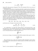
3.2.2 General Heat Conduction Equations
The general equations of heat conduction in the rectangular, cylindrical, and spherical
coordinate systems shown in Fig. 3.1 can be derived by performing an energy balance.
Cartesian coordinate system:
∂
∂x

k
∂T
∂x

+
∂
∂y

k
∂T
∂y

+
∂
∂z

k
∂T
∂z


+˙q = ρc
∂T
∂t
(3.4)
Cylindrical coordinate system:
1
r
∂
∂r

kr
∂T
∂r

+
1
r
2
∂
∂φ

k
∂T
∂φ

+
∂
∂z


k
∂T
∂z

+˙q = ρc
∂T
∂t
(3.5)
Spherical coordinate system:
1
r
2
∂
∂r

kr
2
∂T
∂r

+
1
r
2
sin
2
θ
∂
∂φ


k
∂T
∂φ

+
1
r
2
sin θ
∂
∂θ

k sin θ
∂T
∂θ

+˙q = ρc
∂T
∂t
(3.6)
In eqs. (3.4)–(3.6), ˙q is the volumetric energy addition (W/m
3
), ρ the density of
the material (kg/m
3
), and c the specific heat (J/kg ·K) of the material. The general
heat conduction equation can also be expressed in a general curvilinear coordinate
system (Section 1.2.4). Ozisik (1993) gives the heat conduction equations in prolate
spheroidal and oblate spheroidal coordinate systems.
3.2.3 Boundary and Initial Conditions

Each of the general heat conduction equations (3.4)–(3.6) is second order in the
spatial coordinates and first order in time. Hence, the solutions require a total of six
BOOKCOMP, Inc. — John Wiley & Sons / Page 166 / 2nd Proofs / Heat Transfer Handbook / Bejan
166 CONDUCTION HEAT TRANSFER
1
2
3
4
5
6
7
8
9
10
11
12
13
14
15
16
17
18
19
20
21
22
23
24
25
26

27
28
29
30
31
32
33
34
35
36
37
38
39
40
41
42
43
44
45
[166], (6)
Lines: 372 to 379
———
0.951pt PgVar
———
Long Page
* PgEnds: Eject
[166],
(6)
q
zdzϩ

q
zdzϩ
q
ydyϩ
q
xdxϩ
q
dϩ␪␪
q
␾ϩ ␾d
q
␾ϩ ␾d
q
rdrϩ
q
rdrϩ
q
␪
q
y
q
z
q
r
q
z
q
␾
q
x

q
␾
dz
dy
dx
z
y
x
rd␾
rd␪
dz
dr
z
r
z
x
x
y
y
␾
␾
Tr z(, ,)␾
Tr(, , )␾␪
dr
r
d
sin
␾
␪
␪

r
()a ()c
()b
Figure 3.1 Differential control volumes in (a) Cartesian, (b) cylindrical, and (c) spherical
coordinates.
boundary conditions (two for each spatial coordinate) and one initial condition. The
initial condition prescribes the temperature in the body at time t = 0. The three
types of boundary conditions commonly encountered are that of constant surface
temperature (the boundary condition of the first kind), constant surface heat flux (the
boundary condition of the second kind), and a prescribed relationship between the
surface heat flux and the surface temperature (the convective or boundary condition
of the third kind). The precise mathematical form of the boundary conditions depends
on the specific problem.
For example, consider one-dimensional transient condition in a semi-infinite solid
that is subject to heating at x = 0. Depending on the characterization of the heating,
the boundary condition at x = 0 may take one of three forms. For constant surface
temperature,
BOOKCOMP, Inc. — John Wiley & Sons / Page 167 / 2nd Proofs / Heat Transfer Handbook / Bejan
SPECIAL FUNCTIONS
167
1
2
3
4
5
6
7
8
9
10

11
12
13
14
15
16
17
18
19
20
21
22
23
24
25
26
27
28
29
30
31
32
33
34
35
36
37
38
39
40

41
42
43
44
45
[167], (7)
Lines: 379 to 443
———
0.24222pt PgVar
———
Long Page
* PgEnds: Eject
[167],
(7)
T(0,t)= T
s
(3.7)
For constant surface heat flux,
− k
∂T(0,t)
∂x
= q

s
(3.8)
and for convection at x = 0,
− k
∂T(0,t)
∂x
= h

[
T
∞
− T(0,t)
]
(3.9)
where in eq. (3.9), h(W/m
2
·K) is the convective heat transfer coefficient and T
∞
is
the temperature of the hot fluid in contact with the surface at x = 0.
Besides the foregoing boundary conditions of eqs. (3.7)–(3.9), other types of
boundary conditions may arise in heat conduction analysis. These include bound-
ary conditions at the interface of two different materials in perfect thermal contact,
boundary conditions at the interface between solid and liquid phases in a freezing
or melting process, and boundary conditions at a surface losing (or gaining) heat
simultaneously by convection and radiation. Additional details pertaining to these
boundary conditions are provided elsewhere in the chapter.
3.3 SPECIAL FUNCTIONS
A number of special mathematical functions frequently arise in heat conduction anal-
ysis. These cannot be computed readily using a scientific calculator. In this section
we provide a modest introduction to these functions and their properties. The func-
tions include error functions, gamma functions, beta functions, exponential integral
functions, Bessel functions, and Legendre polynomials.
3.3.1 Error Functions
The error function with argument (x) is defined as
erf(x) =
2
√

π

x
0
e
−t
2
dt (3.10)
where t is a dummy variable. The error function is an odd function, so that
erf(−x) =−erf(x) (3.11)
In addition,
erf(0) = 0 and erf(∞) = 1 (3.12)
The complementary error function with argument (x) is defined as
erfc(x) = 1 − erf(x) =
2
√
π

∞
x
e
−t
2
dt (3.13)
BOOKCOMP, Inc. — John Wiley & Sons / Page 168 / 2nd Proofs / Heat Transfer Handbook / Bejan
168 CONDUCTION HEAT TRANSFER
1
2
3
4

5
6
7
8
9
10
11
12
13
14
15
16
17
18
19
20
21
22
23
24
25
26
27
28
29
30
31
32
33
34

35
36
37
38
39
40
41
42
43
44
45
[168], (8)
Lines: 443 to 598
———
0.81136pt PgVar
———
Normal Page
PgEnds: T
E
X
[168],
(8)
The derivatives of the error function can be obtained by repeated differentiations
of eq. (3.10):
d
dx
erf(x) =
2
√
π

e
−x
2
and
d
2
dx
2
erf(x) =−
4
√
π
xe
−x
2
(3.14)
The repeated integrals of the complementary error function are defined by
i
n
erfc(x) =

∞
x
i
n−1
erfc(t) dt (n = 1, 2, 3, ) (3.15)
with
i
0
erfc(x) = erfc(x) and i

−1
erfc(x) =
2
√
π
e
−x
2
(3.16)
The first two repeated integrals are
i erfc(x) =
1
√
π
e
−x
2
− x erfc(x) (3.17)
i
2
erfc(x) =
1
4


1 + 2x
2

erfc(x) −
2

√
π
xe
−x
2

(3.18)
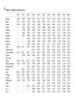
Table 3.1 lists the values of erf(x), d erf(x)/dx, d
2
erf(x)/dx
2
, and d
3
erf(x)/dx
3
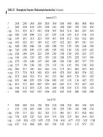
for values of x from 0 to 3 in increments of 0.10. Table 3.2 lists the values of
erfc(x), i erfc(x), i
2
erfc(x), and i
3
erfc(x) for the same values of x. Both tables
were generated using Maple V (Release 6.0).
3.3.2 Gamma Function
The gamma function, denoted by Γ(x), provides a generalization of the factorial n!
to the case where n is not an integer. It is defined by the Euler integral (Andrews,
1992):
Γ(x) =

∞
0

t
x−1
e
−t
dt (x > 0) (3.19)
and has the property
Γ(x + 1) = xΓ(x) (3.20)
which for integral values of x (denoted by n) becomes
Γ(n + 1) = n! (3.21)
Table 3.3 gives values of Γ(x) for values of x from 1.0 through 2.0. These values
were generated using Maple V, Release 6.0.
BOOKCOMP, Inc. — John Wiley & Sons / Page 169 / 2nd Proofs / Heat Transfer Handbook / Bejan
SPECIAL FUNCTIONS
169
1
2
3
4
5
6
7
8
9
10
11
12
13
14
15
16

17
18
19
20
21
22
23
24
25
26
27
28
29
30
31
32
33
34
35
36
37
38
39
40
41
42
43
44
45
[169], (9)

Lines: 598 to 618
———
0.85535pt PgVar
———
Normal Page
* PgEnds: Eject
[169],
(9)
TABLE 3.1 Values of erf(x), d erf(x)/dx, d
2
erf(x)/dx
2
, and d
3
erf(x)/dx
3
x erf(x) d erf(x)/dx d
2
erf(x)/dx
2
d
3
erf(x)/dx
3
0.00 0.00000 1.12838 0.00000 −2.25676
0.10 0.11246 1.11715 −0.22343 −2.18962
0.20 0.22270 1.08413 −0.43365 −1.99481
0.30 0.32863 1.03126 −0.61876 −1.69127
0.40 0.42839 0.96154 −0.76923 −1.30770
0.50 0.52050 0.87878 −0.87878 −0.87878

0.60 0.60386 0.78724 −0.94469 −0.44086
0.70 0.67780 0.69127 −0.96778 −0.02765
0.80 0.74210 0.59499 −0.95198 0.33319
0.90 0.79691 0.50197 −0.90354 0.62244
1.00 0.84270 0.41511 −0.83201 0.83021
1.10 0.88021 0.33648 −0.74026 0.95560
1.20 0.91031 0.26734 −0.64163 1.00521
1.30 0.93401 0.20821 −0.54134 0.99107
1.40 0.95229 0.15894 −0.44504 0.92822
1.50 0.96611 0.11893 −0.35679 0.83251
1.60 0.97635 0.08723 −0.27913 0.71877
1.70 0.98379 0.06271 −0.21322 0.59952
1.80 0.98909 0.04419 −0.15909 0.48434
1.90 0.99279 0.03052 −0.11599 0.37973
2.00 0.99532 0.02067 −0.08267 0.28934
2.10 0.99702 0.01372 −0.05761 0.21451
2.20 0.99814 0.00892 −0.03926 0.15489
2.30 0.99886 0.00569 −0.02617 0.10900
2.40 0.99931 0.00356 −0.01707 0.07481
2.50 0.99959 0.00218 −0.01089 0.05010
2.60 0.99976 0.00131 −0.00680 0.03275
2.70 0.99987 0.76992 ×10
−3
−0.00416 0.02091
2.80 0.99992 0.44421 ×10
−3
−0.00249 0.01305
2.90 0.99996 0.25121 ×10
−3
−0.00146 0.00795

3.00 0.99997 0.13925 ×10
−3
−0.83552 ×10
−3
0.00473
The incomplete gamma function is defined by the integral (Andrews, 1992)
Γ(a, x) =

∞
x
t
a−1
e
−t
dt (3.22)
Values of Γ(1.2,x)for 0 ≤ x ≤ 1 generated using Maple V, Release 6.0 are given in
Table 3.4.
3.3.3 Beta Functions
The beta function, denoted by B(x,y), is defined by
B(x,y) =

1
0
(1 − t)
x−1
t
y−1
dt (3.23)
BOOKCOMP, Inc. — John Wiley & Sons / Page 170 / 2nd Proofs / Heat Transfer Handbook / Bejan
170 CONDUCTION HEAT TRANSFER

1
2
3
4
5
6
7
8
9
10
11
12
13
14
15
16
17
18
19
20
21
22
23
24
25
26
27
28
29
30

31
32
33
34
35
36
37
38
39
40
41
42
43
44
45
[170], (10)
Lines: 618 to 706
———
-0.49988pt PgVar
———
Normal Page
* PgEnds: Eject
[170],
(10)
TABLE 3.2 Values of erfc(x), i erfc(x), i
2
erfc(x), and i
3
erfc(x)
x erfc(x) i erfc(x) i

2
erfc(x) i
3
erfc(x)
0.00 1.00000 0.56419 0.25000 0.09403
0.10 0.88754 0.46982 0.19839 0.07169
0.20 0.77730 0.38661 0.15566 0.05406
0.30 0.67137 0.31422 0.12071 0.04030
0.40 0.57161 0.25213 0.09248 0.02969
0.50 0.47950 0.19964 0.06996 0.02161
0.60 0.39614 0.15594 0.05226 0.01554
0.70 0.32220 0.12010 0.03852 0.01103
0.80 0.25790 0.09117 0.02801 0.00773
0.90 0.20309 0.06820 0.02008 0.00534
1.00 0.15730 0.05025 0.01420 0.00364
1.10 0.11979 0.03647 0.00989 0.00245
1.20 0.08969 0.02605 0.00679 0.00162
1.30 0.06599 0.01831 0.00459 0.00106
1.40 0.04771 0.01267 0.00306 0.68381 × 10
−3
1.50 0.03389 0.00862 0.00201 0.43386 × 10
−3
1.60 0.02365 0.00577 0.00130 0.27114 × 10
−3
1.70 0.01621 0.00380 0.82298 × 10
−3
0.16686 ×10
−3
1.80 0.01091 0.00246 0.51449 × 10
−3

0.10110 ×10
−3
1.90 0.00721 0.00156 0.31642 × 10
−3
0.60301 ×10
−4
2.00 0.00468 0.97802 ×10
−3
0.19141 ×10
−3
0.35396 ×10
−4
2.10 0.00298 0.60095 ×10
−3
0.11387 ×10
−3
0.20445 ×10
−4
2.20 0.00186 0.36282 ×10
−3
0.66614 ×10
−4
0.11619 ×10
−4
2.30 0.00114 0.21520 ×10
−3
0.38311 ×10
−4
0.64951 ×10
−5

2.40 0.68851 ×10
−3
0.12539 ×10
−3
0.21659 ×10
−4
0.35711 ×10
−5
2.50 0.40695 ×10
−3
0.71762 ×10
−4
0.12035 ×10
−4
0.19308 ×10
−5
2.60 0.23603 ×10
−3
0.40336 ×10
−4
0.65724 ×10
−5
0.10265 ×10
−5
2.70 0.13433 ×10
−3
0.22264 ×10
−4
0.35268 ×10
−5

0.53654 ×10
−6
2.80 0.75013 ×10
−4
0.12067 ×10
−4
0.18595 ×10
−5
0.27567 ×10
−6
2.90 0.41098 ×10
−4
0.64216 ×10
−5
0.96315 ×10
−6
0.13922 ×10
−6
3.00 0.22090 ×10
−4
0.33503 ×10
−5
0.49007 ×10
−6
0.69101 ×10
−7
The beta function is related to the gamma function:
B(x,y) =
Γ(x)Γ(y)
Γ(x + y)

(x > 0,y >0) (3.24)
has the symmetry property
B(x,y) = B(y,x) (3.25)
and for nonnegative integers,
B(m,n) =
(m − 1)!(n − 1)!
(m + n − 1)!
m, n nonnegative integers (3.26)