Heat Transfer Handbook part 20 pdf

BOOKCOMP, Inc. — John Wiley & Sons / Page 181 / 2nd Proofs / Heat Transfer Handbook / Bejan
STEADY ONE-DIMENSIONAL CONDUCTION
181
1
2
3
4
5
6
7
8
9
10
11
12
13
14
15
16
17
18
19
20
21
22
23
24
25
26
27
28

29
30
31
32
33
34
35
36
37
38
39
40
41
42
43
44
45
[181], (21)
Lines: 1105 to 1146
———
2.92108pt PgVar
———
Normal Page
* PgEnds: Eject
[181],
(21)
T
s,1
r
1

r
2
T
s,2
k
L
q
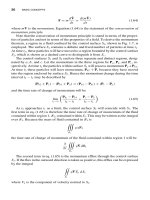
Figure 3.7 Radial conduction through a hollow cylinder.
in the radial direction with no internal heat generation and constant thermal conduc-
tivity, the appropriate form of the general heat conduction equation, eq. (3.5), is
d
dr

r
dT
dr

= 0 (3.69)
with the boundary conditions expressed as
T(r = r
1
) = T
s,1
and T(r = r
2
) = T
s,2
(3.70)
Following the same procedure as that used for the plane wall will give the temperature
distribution

T = T
s,1
+
T
s,1
− T
s,2
ln(r
1
/r
2
)
ln
r
r
1
(3.71)
and the heat flow
q =
2πkL(T
x,1
− T
s,2
)
ln(r
2
/r
1
)
(3.72)

3.4.3 Hollow Sphere
The description pertaining to the hollow cylinder also applies to the hollow sphere
of Fig. 3.8 except that the length L is no longer relevant. The applicable form of eq.
(3.6) is
d
dr

r
2
dT
dr

= 0 (3.73)
BOOKCOMP, Inc. — John Wiley & Sons / Page 182 / 2nd Proofs / Heat Transfer Handbook / Bejan
182 CONDUCTION HEAT TRANSFER
1
2
3
4
5
6
7
8
9
10
11
12
13
14
15

16
17
18
19
20
21
22
23
24
25
26
27
28
29
30
31
32
33
34
35
36
37
38
39
40
41
42
43
44
45

[182], (22)
Lines: 1146 to 1188
———
4.84712pt PgVar
———
Long Page
* PgEnds: Eject
[182],
(22)
Figure 3.8 Radial conduction through a hollow sphere.
with the boundary conditions expressed as
T(r = r
1
) = T
s,1
and T(r = r
2
) = T
s,2
(3.74)
The expressions for the temperature distribution and heat flow are
T = T
s,1
+
T
s,1
− T
s,2
1/r
2

− 1/r
1

1
r
1
−
1
r

(3.75)
q =
4πk(T
s,1
− T
s,2
)
1/r
1
− 1/r
2
(3.76)
3.4.4 Thermal Resistance
Thermal resistance is defined as the ratio of the temperature difference to the associ-
ated rate of heat transfer. This is completely analogous to electrical resistance, which,
according to Ohm’s law, is defined as the ratio of the voltage difference to the current
flow. With this definition, the thermal resistance of the plane wall, the hollow cylinder,
and the hollow sphere are, respectively,
R
cond

=
L
kA
(3.77)
R
cond
=
ln(r
2
/r
1
)
2πkL
(3.78)
R
cond
=
1/r
1
− 1/r
2
4πk
(3.79)
BOOKCOMP, Inc. — John Wiley & Sons / Page 183 / 2nd Proofs / Heat Transfer Handbook / Bejan
STEADY ONE-DIMENSIONAL CONDUCTION
183
1
2
3
4

5
6
7
8
9
10
11
12
13
14
15
16
17
18
19
20
21
22
23
24
25
26
27
28
29
30
31
32
33
34

35
36
37
38
39
40
41
42
43
44
45
[183], (23)
Lines: 1188 to 1259
———
0.37024pt PgVar
———
Long Page
* PgEnds: Eject
[183],
(23)
When convection occurs at the boundaries of a solid, it is convenient to define the
convection resistance from Newton’s law of cooling:
q = hA(T
s
− T
∞
) (3.80)
where h is the convection heat transfer coefficient and T
∞
is the convecting fluid

temperature. It follows from eq. (3.80) that
R
conv
=
T
s
− T
∞
q
=
1
hA
(3.81)
3.4.5 Composite Systems
The idea of thermal resistance is a useful tool for analyzing conduction through
composite members.
Composite Plane Wall For the series composite plane wall and the associated
thermal network shown in Fig. 3.9, the rate of heat transfer q is given by
q =
T
∞,1
− T
∞,2
1/h
1
A + L
1
/k
1
A + L

2
/k
2
A + 1/h
2
A
(3.82)
Once q has been determined, the surface and interface temperatures can be found:
T
s,1
= T
∞,1
− q
1
h
1
A
(3.83)
T
2
= T
∞,1
− q

1
h
1
A
+
L

1
k
1
A

(3.84)
T
s,2
= T
∞,1
− q

1
h
1
A
+
L
1
k
1
A
+
L
2
k
2
A

(3.85)

Figure 3.10 illustrates a series–parallel composite wall. If materials 2 and 3 have
comparable thermal conductivities, the heat flow may be assumed to be one-dimen-
sional. The network shown in Fig. 3.10 assumes that surfaces normal to the direction
of heat flow are isothermal. For a wall of unit depth, the heat transfer rate is
q =
T
s,1
− T
s,2
L
1
/k
1
H
1
+ L
2
L
3
/(k
2
H
2
L
3
+ k
3
H
3
L

2
) + L
4
/k
4
H
4
(3.86)
where H
1
= H
2
+H
3
= H
4
and the rule for combining resistances in parallel has been
employed. Once q has been determined, the interface temperatures may be computed:
T
1
= T
s,1
− q
L
1
k
1
H
1
(3.87)

T
2
= T
s,2
+ q
L
4
k
4
H
4
(3.88)
BOOKCOMP, Inc. — John Wiley & Sons / Page 184 / 2nd Proofs / Heat Transfer Handbook / Bejan
184 CONDUCTION HEAT TRANSFER
1
2
3
4
5
6
7
8
9
10
11
12
13
14
15
16

17
18
19
20
21
22
23
24
25
26
27
28
29
30
31
32
33
34
35
36
37
38
39
40
41
42
43
44
45
[184], (24)

Lines: 1259 to 1259
———
*
35.45401pt PgVar
———
Normal Page
PgEnds: T
E
X
[184],
(24)
Figure 3.9 Series composite wall and its thermal network.
T
s,1
L
1
H
1
H
3
L
1
k
1
L
2
H
2
L
3

L
3
L
4
L
4
H
4
L
2
k
2
k
3
k
4
T
2
T
2
T
1
T
1
T
s,2
T
s,1
T
s,2

kH
11
kH
22
kH
44
kH
33
q
Figure 3.10 Series–parallel composite wall and its thermal network.
BOOKCOMP, Inc. — John Wiley & Sons / Page 185 / 2nd Proofs / Heat Transfer Handbook / Bejan
STEADY ONE-DIMENSIONAL CONDUCTION
185
1
2
3
4
5
6
7
8
9
10
11
12
13
14
15
16
17

18
19
20
21
22
23
24
25
26
27
28
29
30
31
32
33
34
35
36
37
38
39
40
41
42
43
44
45
[185], (25)
Lines: 1259 to 1286

———
1.82707pt PgVar
———
Normal Page
PgEnds: T
E
X
[185],
(25)
T
s,1
T
s,1
k
1
r
1
k
2
r
2
r
3
T
2
T
2
T
s,2
T

s,2
T
ϱ1
T
ϱ2
hrL
11
2␲ hrL
2
3
2␲2 kL
1
␲ 2 kL
2
␲
ln r r(/)
21
ln r r(/)
32
L
q
11
Cold fluid
,Th
ϱ22
Hot fluid
,Th
ϱ11
Figure 3.11 Series composite hollow cylinder and its thermal network.
Composite Hollow Cylinder A typical composite hollow cylinder with both

inside and outside experiencing convection is shown in Fig. 3.11. The figure includes
the thermal network that represents the system. The rate of heat transfer q is given by
q =
T
∞,1
− T
∞,2
1/2πh
1
r
1
L + ln(r
2
/r
1
)/2πk
1
L + ln(r
3
/r
2
)/2πk
2
L + 1/2πh
2
r
3
L
(3.89)
Once q has been determined, the inside surface T

s,1
, the interface temperature T
2
, and
the outside surface temperature T
s,2
can be found:
T
s,1
= T
∞,1
− q
1
2πh
1
r
1
L
(3.90)
BOOKCOMP, Inc. — John Wiley & Sons / Page 186 / 2nd Proofs / Heat Transfer Handbook / Bejan
186 CONDUCTION HEAT TRANSFER
1
2
3
4
5
6
7
8
9

10
11
12
13
14
15
16
17
18
19
20
21
22
23
24
25
26
27
28
29
30
31
32
33
34
35
36
37
38
39

40
41
42
43
44
45
[186], (26)
Lines: 1286 to 1307
———
3.39914pt PgVar
———
Normal Page
* PgEnds: Eject
[186],
(26)
T
2
= T
∞,1
− q

1
2πh
1
r
1
L
+
ln(r
2

/r
1
)
2πk
1
L

(3.91)
T
s,2
= T
∞,2
+ q
1
2πh
2
r
3
L
(3.92)
Composite Hollow Sphere Figure 3.12 depicts a composite hollow sphere
made of two layers and experiencing convective heating on the inside surface and
convective cooling on the outside surface. From the thermal network, also shown in
Fig. 3.12, the rate of heat transfer q can be determined as
q =
T
∞,1
− T
∞,2
1/4πh

1
r
2
1
+ (r
2
− r
1
)/4πk
1
r
1
r
2
+ (r
3
− r
2
)/4πk
2
r
3
r
2
+ 1/4πh
2
r
2
3
(3.93)

Once q has been determined, temperatures T
s,1
,T
2
, and T
s,2
can be found:
T
s,1
T
s,1
T
s,1
k
1
r
1
k
2
r
2
r
3
T
2
T
2
T
s,2
T

ϱ1
q
T
ϱ2
hr
1
1
2
4␲ hr
2
3
2
4␲4 k
1
␲ 4 k
2
␲
1/ 1/rr
12
Ϫ 1/ 1/rr
23
Ϫ
q
11
Cold fluid
,Th
ϱ22
Hot fluid
,Th
ϱ11

Figure 3.12 Series composite hollow sphere and its thermal network.
BOOKCOMP, Inc. — John Wiley & Sons / Page 187 / 2nd Proofs / Heat Transfer Handbook / Bejan
STEADY ONE-DIMENSIONAL CONDUCTION
187
1
2
3
4
5
6
7
8
9
10
11
12
13
14
15
16
17
18
19
20
21
22
23
24
25
26

27
28
29
30
31
32
33
34
35
36
37
38
39
40
41
42
43
44
45
[187], (27)
Lines: 1307 to 1334
———
0.55927pt PgVar
———
Normal Page
PgEnds: T
E
X
[187],
(27)

T
s,1
= T
∞,1
− q
1
4πh
1
r
2
1
(3.94)
T
2
= T
∞,1
− q

1
4πh
1
r
2
1
+
1
4πk
1

1

r
1
−
1
r
2

(3.95)
T
s,2
= T
∞,2
+ q
1
4πh
2
r
2
3
(3.96)
3.4.6 Contact Conductance
The heat transfer analyses for the composite systems described in Section 3.4.5 as-
sumed perfect contact at the interface between the two materials. In reality, how-
ever, the mating surfaces are rough and the actual contact occurs at discrete points
(asperities or peaks), as indicated in Fig. 3.13. The gaps of voids are usually filled
with air, and the heat transfer at the interface is the sum of solid conduction across
the contact points and fluid conduction through the gaps. Because of the imperfect
contact, there is a temperature drop across the gap or interface, ∆T
c
. The contact

conductance h
c
(W/m
2
·K) is defined as the ratio of the heat flux q/A through the
interface to the interface temperature drop:
h
c
=
q/A
∆T
c
=
1
R

c
(3.97)
where q/A is the heat flux through the interface and R

c
(m
2
·K/W), the inverse of h
c
,
is the contact resistance.
The topic of contact conductance is of considerable contemporary interest, as
reflected by a review paper of Fletcher (1988), a book by Madhusudana (1996),
Figure 3.13 Contact interface for actual surfaces.

BOOKCOMP, Inc. — John Wiley & Sons / Page 188 / 2nd Proofs / Heat Transfer Handbook / Bejan
188 CONDUCTION HEAT TRANSFER
1
2
3
4
5
6
7
8
9
10
11
12
13
14
15
16
17
18
19
20
21
22
23
24
25
26
27
28

29
30
31
32
33
34
35
36
37
38
39
40
41
42
43
44
45
[188], (28)
Lines: 1334 to 1377
———
1.12001pt PgVar
———
Short Page
PgEnds: T
E
X
[188],
(28)
and numerous contributions from several research groups. Chapter 4 of this book
is devoted exclusively to this subject.

3.4.7 Critical Thickness of Insulation
When a plane surface is covered with insulation, the rate of heat transfer always
decreases. However, the addition of insulation to a cylindrical or spherical surface
increases the conduction resistance but reduces the convection resistance because
of the increased surface area. The critical thickness of insulation corresponds to the
condition when the sum of conduction and convection resistances is a minimum. For
a given temperature difference, this results in a maximum heat transfer rate, and the
critical radius r
c
is given by
r
c
=

k
h
(cylinder) (3.98)
2k
h
(sphere) (3.99)
where k is the thermal conductivity of the insulation and h is the convective heat
transfer coefficient for the outside surface.
The basic analysis for obtaining the critical radius expression has been modified
to allow for:
• The variation of h with outside radius
• The variation of h with outside radius, including the effect of temperature-
dependent fluid properties
• Circumferential variation of h
• Pure radiation cooling
• Combined natural convection and radiation cooling

The analysis for a circular pipe has also been extended to include insulation
boundaries that form equilateral polygons, rectangles, and concentric circles. Such
configurations require a two-dimensional conduction analysis and have led to the
conclusion that the concept of critical perimeter of insulation, P
c
= 2π(k/h),is
more general than that of critical radius. The comprehensive review article by Aziz
(1997) should be consulted for further details.
3.4.8 Effect of Uniform Internal Energy Generation
In some engineering systems, it becomes necessary to analyze one-dimensional steady
conduction with internal energy generation. Common sources of energy generation
are the passage of an electric current through a wire or busbar or a rear window
defroster in an automobile. In the fuel element of a nuclear reactor, the energy is
generated due to neutron absorption. A vessel containing nuclear waste experiences
energy generation as the waste undergoes a slow process of disintegration.
BOOKCOMP, Inc. — John Wiley & Sons / Page 189 / 2nd Proofs / Heat Transfer Handbook / Bejan
STEADY ONE-DIMENSIONAL CONDUCTION
189
1
2
3
4
5
6
7
8
9
10
11
12

13
14
15
16
17
18
19
20
21
22
23
24
25
26
27
28
29
30
31
32
33
34
35
36
37
38
39
40
41
42

43
44
45
[189], (29)
Lines: 1377 to 1420
———
0.18512pt PgVar
———
Short Page
PgEnds: T
E
X
[189],
(29)
Plane Wall Consider first a plane wall of thickness 2L, made of a material having
a thermal conductivity k, as shown in Fig. 3.14. The volumetric rate of energy gener-
ation in the wall is ˙q (W/m
3
). Let T
s,1
and T
s,2
be the two surface temperatures, and
assuming the thermal conductivity of the wall to be constant, the appropriate form of
eq. (3.4) is
d
2
T
dx
2

+
˙q
k
= 0 (3.100)
and the boundary conditions are
T(x=−L) = T
s,1
and T(x= L) = T
s,2
(3.101)
The solution for the temperature distribution is
T =
˙q
2k

L
2
− x
2

+
T
s,2
− T
s,1
2L
x +
T
s,2
+ T

s,1
2
(3.102)
The maximum temperature occurs at x = k(T
s,2
− T
s,1
)/2L ˙q and is given by
T
max
=
˙qL
2
2k
+
k(T
s,2
− T
s,1
)
2
8 ˙qL
2
+
T
s,2
+ T
s,1
2
(3.103)

If the face at x =−L is cooled by convection with a heat transfer coefficient h
1
and
coolant temperature T
∞,1
, and the face at x =+L is cooled by convection with a
heat transfer coefficient h
2
and coolant temperature T
∞,2
, the overall energy balance
gives
2 ˙qL = h
1
(T
s,1
− T
∞,1
) + h
2
(T
s,2
− T
∞,2
) (3.104)
T
s,1
T
s,2
q

hT
1,1
,
ϱ
hT
2,2
,
ϱ
ϪL ϩL
x
.
Figure 3.14 Conduction in a plane wall with uniform internal energy generation.
BOOKCOMP, Inc. — John Wiley & Sons / Page 190 / 2nd Proofs / Heat Transfer Handbook / Bejan
190 CONDUCTION HEAT TRANSFER
1
2
3
4
5
6
7
8
9
10
11
12
13
14
15
16

17
18
19
20
21
22
23
24
25
26
27
28
29
30
31
32
33
34
35
36
37
38
39
40
41
42
43
44
45
[190], (30)

Lines: 1420 to 1465
———
-1.06888pt PgVar
———
Normal Page
PgEnds: T
E
X
[190],
(30)
When T
s,1
= T
s,2
, the temperature distribution is symmetrical about x = 0 and is
given by
T =
˙q
2k

L
2
− x
2

+ T
s
(3.105)
and the maximum temperature occurs at the midplane (x = 0), which can be ex-
pressed as

T
max
=
˙qL
2
2k
+ T
s
(3.106)
When T
∞,1
= T
∞,2
= T
∞
and h
1
= h
2
= h, eq. (3.104) reduces to
T
s
− T
∞
=
˙qL
h
(3.107)
Hollow Cylinder For the hollow cylinder shown in Fig. 3.15, the appropriate form
of eq. (3.5) for constant k is

1
r
d
dr

r
dT
dr

+
˙q
k
= 0 (3.108)
and the boundary conditions are
T(r = r
1
) = T
s,1
and T(r = r
2
) = T
s,2
(3.109)
T
s,1
r
1
r
2
r

k
T
s,2
L
q
Cold fluid
,Th
ϱ,2 2
Cold fluid
,Th
ϱ,1 1
.
Figure 3.15 Conduction in a hollow cylinder with uniform internal energy generation.