Electric Circuits, 9th Edition P4 pdf

engineering a challenging and exciting profession. The emphasis in engi-
neering is on making things work, so an engineer is free to acquire and
use any technique, from any field, that helps to get the job done.
Circuit Theory
In a field as diverse as electrical engineering, you might well ask whether
all of its branches have anything in common. The answer is yes—electric
circuits. An electric circuit is a mathematical model that approximates
the behavior of an actual electrical system. As such, it provides an impor-
tant foundation for learning—in your later courses and as a practicing
engineer—the details of how to design and operate systems such as those
just described. The models, the mathematical techniques, and the language
of circuit theory will form the intellectual framework for your future engi-
neering endeavors.
Note that the term electric circuit is commonly used to refer to an
actual electrical system as well as to the model that represents it. In this
text, when we talk about an electric circuit, we always mean a model,
unless otherwise stated. It is the modeling aspect of circuit theory that has
broad applications across engineering disciplines.
Circuit theory
is
a special case of electromagnetic field theory: the study
of static and moving electric charges. Although generalized field theory
might seem to be an appropriate starting point for investigating electric sig-
nals,
its application is not only cumbersome but also requires the use of
advanced mathematics. Consequently, a course in electromagnetic field
theory is not a prerequisite to understanding the material in this book. We
do,
however, assume that you have had an introductory physics course in
which electrical and magnetic phenomena were discussed.
Three basic assumptions permit us to use circuit theory, rather than

electromagnetic field theory, to study a physical system represented by an
electric circuit. These assumptions are as follows:
1.
Electrical effects happen instantaneously throughout a system. We
can make this assumption because we know that electric signals
travel at or near the speed of light. Thus, if the system is physically
small, electric signals move through it so quickly that we can con-
sider them to affect every point in the system simultaneously. A sys-
tem that is small enough so that we can make this assumption is
called a lumped-parameter system.
2.
The net charge on every component in the system is always zero.
Thus no component can collect a net excess of charge, although
some components, as you will learn later, can hold equal but oppo-
site separated charges.
3.
There is no magnetic coupling between the components in a system.
As we demonstrate later, magnetic coupling can occur within a
component.
That's it; there are no other assumptions. Using circuit theory provides
simple solutions (of sufficient accuracy) to problems that would become
hopelessly complicated if we were to use electromagnetic field theory.
These benefits are so great that engineers sometimes specifically design
electrical systems to ensure that these assumptions are met. The impor-
tance of assumptions 2 and 3 becomes apparent after we introduce the
basic circuit elements and the rules for analyzing interconnected elements.
However, we need to take a closer look at assumption l.The question
is,
"How small does a physical system have to be to qualify as a lumped-
parameter system?" We can get a quantitative handle on the question by

noting that electric signals propagate by wave phenomena. If the wave-
length of the signal is large compared to the physical dimensions of the
system, we have a lumped-parameter system. The wavelength A is the
velocity divided by the repetition rate, or frequency, of the signal; that is,
A = c/f. The frequency /is measured in hertz (Hz). For example, power
systems in the United States operate at 60 Hz. If we use the speed of light
(c = 3 X 10
8
m/s) as the velocity of propagation, the wavelength is
5 X 10
6
m. If the power system of interest is physically smaller than this
wavelength, we can represent it as a lumped-parameter system and use cir-
cuit theory to analyze its behavior. How do we define smaller? A good rule
is the rule of 1/lOth: If the dimension of the system is l/10th (or smaller)
of the dimension of the wavelength, you have a lumped-parameter system.
Thus,
as long as the physical dimension of the power system is less than
5 X 10
5
m, we can treat it as a lumped-parameter system.
On the other hand, the propagation frequency of radio signals is on the
order of 10
9
Hz.Thus the wavelength is 0.3 m. Using the rule of l/10th, the
relevant dimensions of a communication system that sends or receives radio
signals must be less than 3 cm to qualify as a lumped-parameter system.
Whenever any of the pertinent physical dimensions of a system under study
approaches the wavelength of its signals, we must use electromagnetic field
theory to analyze that system. Throughout this book we study circuits

derived from lumped-parameter systems.
Problem Solving
As a practicing engineer, you will not be asked to solve problems that
have already been solved. Whether you are trying to improve the per-
formance of an existing system or creating a new system, you will be work-
ing on unsolved problems. As a student, however, you will devote much of
your attention to the discussion of problems already solved. By reading
about and discussing how these problems were solved in the past, and by
solving related homework and exam problems on your own, you will
begin to develop the skills to successfully attack the unsolved problems
you'll face as a practicing engineer.
Some general problem-solving procedures are presented here. Many
of them pertain to thinking about and organizing your solution strategy
before proceeding with calculations.
1.
Identify what's given and what's to be
found.
In problem solving, you
need to know your destination before you can select a route for get-
ting there. What is the problem asking you to solve or find?
Sometimes the goal of the problem is obvious; other times you may
need to paraphrase or make lists or tables of known and unknown
information to see your objective.
The problem statement may contain extraneous information
that you need to weed out before proceeding. On the other hand, it
may offer incomplete information or more complexities than can be
handled given the solution methods at your disposal. In that case,
you'll need to make assumptions to fill in the missing information or
simplify the problem context. Be prepared to circle back and recon-
sider supposedly extraneous information and/or your assumptions if

your calculations get bogged down or produce an answer that doesn't
seem to make sense.
2.
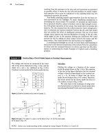
Sketch a circuit diagram or other visual model. Translating a verbal
problem description into a visual model is often a useful step in the
solution process. If a circuit diagram is already provided, you may
need to add information to it, such as labels, values, or reference
directions. You may also want to redraw the circuit in a simpler, but
equivalent, form. Later in this text you will learn the methods for
developing such simplified equivalent circuits.
3.
Think of several solution methods and decide on a way of choosing
among them. This course will help you build a collection of analyt-
ical tools, several of which may work on a given problem. But one
method may produce fewer equations to be solved than another,
or it may require only algebra instead of calculus to reach a solu-
tion. Such efficiencies, if you can anticipate them, can streamline
your calculations considerably. Having an alternative method in
mind also gives you a path to pursue if your first solution attempt
bogs down.
4.
Calculate a solution. Your planning up to this point should have
helped you identify a good analytical method and the correct equa-
tions for the problem. Now comes the solution of those equations.
Paper-and-pencil, calculator, and computer methods are all avail-
able for performing the actual calculations of circuit analysis.
Efficiency and your instructor's preferences will dictate which tools
you should use.
5.
Use

your creativity. If you suspect that your answer is off base or if the
calculations seem to go on and on without moving you toward a solu-
tion, you should pause and consider alternatives. You may need to
revisit your assumptions or select a different solution method. Or, you
may need to take a less-conventional problem-solving approach, such
as working backward from a solution. This text provides answers to all
of the Assessment Problems and many of the Chapter Problems so
that you may work backward when you get stuck. In the real world,
you won't be given answers in advance, but you may have a desired
problem outcome in mind from which you can work backward. Other
creative approaches include allowing yourself to see parallels with
other types of problems you've successfully solved, following your
intuition or hunches about how to proceed, and simply setting the
problem aside temporarily and coming back to it later.
6. Test your solution. Ask yourself whether the solution you've
obtained makes sense. Does the magnitude of the answer seem rea-
sonable? Is the solution physically realizable? You may want to go
further and rework the problem via an alternative method. Doing
so will not only test the validity of your original answer, but will also
help you develop your intuition about the most efficient solution
methods for various kinds of problems. In the real world, safety-
critical designs are always checked by several independent means.
Getting into the habit of checking your answers will benefit you as
a student and as a practicing engineer.
These problem-solving steps cannot be used as a recipe to solve every prob-
lem in this or any other course. You may need to skip, change the order of,
or elaborate on certain steps to solve a particular problem. Use these steps
as a guideline to develop a problem-solving style that works for you.
1.2 The International System of Units
Engineers compare theoretical results to experimental results and com-

pare competing engineering designs using quantitative measures. Modern
engineering is a multidisciplinary profession in which teams of engineers
work together on projects, and they can communicate their results in a
meaningful way only if they all use the same units of measure. The
International System of Units (abbreviated SI) is used by all the major
engineering societies and most engineers throughout the world; hence we
use it in this book.
1.2
The
International
System
of Units 9
TABLE 1.1 The International System of Units (SI)
Quantity
Length
Mass
Time
Electric current
Thermodynamic temperature
Amount of substance
Luminous intensity
Basic Unit
meter
kilogram
second
ampere
degree kelvin
mole
candela
Symbol

m
kg
s
A
K
mol
cd
The SI units are based on seven defined quantities:
• length
• mass
• time
• electric current
• thermodynamic temperature
• amount of substance
• luminous intensity
These quantities, along with the basic unit and symbol for each, are
listed in Table
1.1.
Although not strictly SI units, the familiar time units of
minute (60 s), hour (3600 s), and so on are often used in engineering cal-
culations. In addition, defined quantities are combined to form derived
units.
Some, such as force, energy, power, and electric charge, you already
know through previous physics courses. Table 1.2 lists the derived units
used in this book.
In many cases, the SI unit is either too small or too large to use conve-
niently. Standard prefixes corresponding to powers of 10, as listed in
Table 1.3, are then applied to the basic unit. All of these prefixes are cor-
rect, but engineers often use only the ones for powers divisible by 3; thus
centi, deci, deka, and hecto are used

rarely.
Also,
engineers often select the
prefix that places the base number in the range between 1 and 1000.
Suppose that a time calculation yields a result of 10~
5
s, that is, 0.00001 s.
Most engineers would describe this quantity as 10/xs, that is,
10"
5
= 10 X 10"
6
s, rather than as 0.01 ms or 10,000,000 ps.
TABLE 1.2 Derived Units in SI
Quantity
Frequency
Force
Energy or work
Power
Electric charge
Electric potential
Electric resistance
Electric conductance
Electric capacitance
Magnetic flux
Inductance
Unit Name (Symbol)
hertz (Hz)
newton (N)
joule (J)

watt (W)
coulomb (C)
volt (V)
ohm (H)
Siemens (S)
farad (F)
weber (Wb)
henry (H)
TABLE 1.3 Standardized Prefixes to Signify
Powers of 10
Prefix
Formula
s-
1
kg
•
m/s
2
N m
J/s
A-s
J/C
V/A
A/V
C/V
V-s
Wb/A
atto
femto
pico

nano
micro
milli
centi
deci
deka
hecto
kilo
mega
giga
tera
Symbol
a
f
P
n
M
m
c
d
da
h
k
M
G
T
Power
10
-18
io-

15
10"
12
io-
9
10
-6
io-
3
io-
2
io
-1
in
1U
2
in
3
10
6
10
9
10
12
10 Circuit Variables
Example
1.1
illustrates
a
method

for
converting from
one set of
units
to another
and
also uses power-of-ten prefixes.
Example
1.1
Using SI
Units
and Prefixes
for
Powers
of 10
If
a
signal can travel
in a
cable
at
80%
of
the speed
of
light, what length
of
cable, in inches, represents
1
ns?

Therefore,
a
signal traveling
at 80% of the
speed
of
light will cover 9.45 inches
of
cable
in
1
nanosecond.
Solution
First, note that 1
ns =
10
-9
s.
Also, recall that
the
speed
of
Light
c = 3 X
10
8
m/s. Then,
80% of the
speed
of

light
is 0.8c =
(0.8)(3
x 10
8
) =
2.4
x
10
8
m/s. Using
a
product
of
ratios,
we can
convert 80%
of the
speed
of
light from meters-per-
second
to
inches-per-nanosecond.
The
result
is the
distance
in
inches traveled

in
1
ns:
2.4
X
10
8
meters
1 second
100 centimeters
1 inch
1 second 10
y
nanoseconds 1 meter 2.54 centimeters
(2.4
X
10
8
)(100)
(10
9
)(2.54)
= 9.45 inches/nanosecond
I/ASSESSMENT
PROBLEMS
Objective 1—Understand
and be
able
to use SI
units and

the
standard prefixes
for
powers
of 10
1.1
Assume
a
telephone signal travels through
a
cable
at
two-thirds
the
speed
of
light.
How
long
does
it
take
the
signal
to get
from New York
City
to
Miami
if

the distance
is
approximately
1100 miles?
Answer:
8.85 ms.
NOTE: Also
try
Chapter Problems 1.2,1.3,
and
1.4.
1.2 How many dollars
per
millisecond would
the
federal government have
to
collect
to
retire
a
deficit
of
$100 billion
in one
year?
Answer: $3.17/ms.
1.3
Circuit Analysis:
An

Overview
Before becoming involved
in the
details
of
circuit analysis,
we
need
to
take
a
broad look
at
engineering design, specifically
the
design
of
electric
circuits. The purpose
of
this overview
is to
provide
you
with
a
perspective
on where circuit analysis fits within
the
whole

of
circuit design. Even
though this book focuses
on
circuit analysis,
we try to
provide opportuni-
ties
for
circuit design where appropriate.
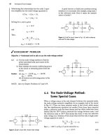
All engineering designs begin with
a
need,
as
shown
in Fig. 1.4.
This
need may come from
the
desire
to
improve
on an
existing design,
or it
may
be something brand-new.
A
careful assessment
of the

need results
in
design specifications, which
are
measurable characteristics
of a
proposed
design. Once
a
design
is
proposed,
the
design specifications allow
us to
assess whether
or not the
design actually meets
the
need.
A concept
for the
design comes next. The concept derives from
a
com-
plete understanding
of
the design specifications coupled with
an
insight into

1.4 Voltage and Current 11
the need, which comes from education and experience. The concept may be
realized as a sketch, as a written description, or in some other form. Often
the next step is to translate the concept into a mathematical model. A com-
monly used mathematical model for electrical systems is a circuit model.
The elements that comprise the circuit model are called ideal circuit
components. An ideal circuit component is a mathematical model of an
actual electrical component, like a battery or a light bulb. It is important
for the ideal circuit component used in a circuit model to represent the
behavior of the actual electrical component to an acceptable degree of
accuracy. The tools of circuit analysis, the focus of this book, are then
applied to the circuit. Circuit analysis is based on mathematical techniques
and is used to predict the behavior of the circuit model and its ideal circuit
components. A comparison between the desired behavior, from the design
specifications, and the predicted behavior, from circuit analysis, may lead
to refinements in the circuit model and its ideal circuit elements. Once the
desired and predicted behavior are in agreement, a physical prototype can
be constructed.
The physical prototype is an actual electrical system, constructed from
actual electrical components. Measurement techniques are used to deter-
mine the actual, quantitative behavior of the physical system. This actual
behavior is compared with the desired behavior from the design specifica-
tions and the predicted behavior from circuit analysis. The comparisons
may result in refinements to the physical prototype, the circuit model, or
both. Eventually, this iterative process, in which models, components, and
systems are continually refined, may produce a design that accurately
matches the design specifications and thus meets the need.
From this description, it is clear that circuit analysis plays a very
important role in the design process. Because circuit analysis is applied to
circuit models, practicing engineers try to use mature circuit models so

that the resulting designs will meet the design specifications in the first
iteration. In this book, we use models that have been tested for between
20 and 100 years; you can assume that they are mature. The ability to
model actual electrical systems with ideal circuit elements makes circuit
theory extremely useful to engineers.
Saying that the interconnection of ideal circuit elements can be used
to quantitatively predict the behavior of a system implies that we can
describe the interconnection with mathematical equations. For the mathe-
matical equations to be useful, we must write them in terms of measurable
quantities. In the case of circuits, these quantities are voltage and current,
which we discuss in Section 1.4. The study of circuit analysis involves
understanding the behavior of each ideal circuit element in terms of its
voltage and current and understanding the constraints imposed on the
voltage and current as a result of interconnecting the ideal elements.
1.4 Voltage and Current
The concept of electric charge is the basis for describing all electrical phe-
nomena. Let's review some important characteristics of electric charge.
• The charge is bipolar, meaning that electrical effects are described in
terms of positive and negative charges.
• The electric charge exists in discrete quantities, which are integral
multiples of the electronic charge,
1.6022
X 10
-19
C.
• Electrical effects are attributed to both the separation of charge and
charges in motion.
In circuit theory, the separation of charge creates an electric force (volt-
age),
and the motion of charge creates an electric fluid (current).

jsjeed
Design
p
h
ysic<iikConc
e
P
l
in*?
1
Circi'
1
.^
analp
rcuit
;r
which
Figure 1.4 • A conceptual model for electrical
engi-
neering design.
12 Circuit Variables
The concepts of voltage and current are useful from an engineering
point of view because they can be expressed quantitatively. Whenever
positive and negative charges are separated, energy is expended. Voltage
is the energy per unit charge created by the separation. We express this
ratio in differential form as
Definition of voltage •
v =
dw
dq '

(1.1)
where
v = the voltage in volts,
w = the energy in joules,
q = the charge in coulombs.
The electrical effects caused by charges in motion depend on the rate
of charge flow. The rate of charge flow is known as the electric current,
which is expressed as
Definition of current •
i =
dq
~di'
(1.2)
where
i = the current in amperes,
q = the charge in coulombs,
t = the time in seconds.
Equations 1.1 and 1.2 are definitions for the magnitude of voltage and
current, respectively. The bipolar nature of electric charge requires that we
assign polarity references to these variables. We will do so in Section 1.5.
Although current is made up of discrete, moving electrons, we do not
need to consider them individually because of the enormous number of
them. Rather, we can think of electrons and their corresponding charge as
one smoothly flowing entity. Thus, i is treated as a continuous variable.
One advantage of using circuit models is that we can model a compo-
nent strictly in terms of the voltage and current at its terminals. Thus two
physically different components could have the same relationship
between the terminal voltage and terminal current. If they do, for pur-
poses of circuit analysis, they are identical. Once we know how a compo-
nent behaves at its terminals, we can analyze its behavior in a circuit.

However, when developing circuit models, we are interested in a compo-
nent's internal behavior. We might want to know, for example, whether
charge conduction is taking place because of free electrons moving
through the crystal lattice structure of a metal or whether it is because of
electrons moving within the covalent bonds of a semiconductor material.
However, these concerns are beyond the realm of circuit theory. In this
book we use circuit models that have already been developed; we do not
discuss how component models are developed.
1.5 The Ideal Basic Circuit Element
An ideal basic circuit element has three attributes: (1) it has only two ter-
minals, which are points of connection to other circuit components; (2) it is
described mathematically in terms of current and/or voltage; and (3) it
cannot be subdivided into other elements. We use the word ideal to imply
1.5
The
Ideal Basic Circuit Element
13
thai a basic circuit element does not exist as a realizable physical compo-
nent. However, as we discussed in Section 1.3, ideal elements can be con-
nected in order to model actual devices and systems. We use the word
basic to imply that ihe circuit element cannot be further reduced or sub-
divided into other
elements.
Thus the basic circuit elements form the build-
ing blocks for constructing circuit models, but they themselves cannot be
modeled with any other type of element.
Figure 1.5 is a representation of an ideal basic circuit element. The box
is blank because we are making no commitment at this time as to the type
of circuit element it is. In Fig. 1.5, the voltage across the terminals of the
box is denoted by v, and the current in the circuit element is denoted by /.

The polarity reference for the voltage is indicated by the plus and minus
signs,
and the reference direction for the current is shown by the arrow
placed alongside the current. The interpretation of these references given
positive or negative numerical values of v and i is summarized in
Table 1.4. Note that algebraically the notion of positive charge flowing in
one direction is equivalent to the notion of negative charge flowing in the
opposite direction.
The assignments of the reference polarity for voltage and the refer-
ence direction for current are entirely arbitrary. However, once you have
assigned the references, you must write all subsequent equations to
agree with the chosen references. The most widely used sign convention
applied to these references is called the passive sign convention, which
we use throughout this book. The passive sign convention can be stated
as follows:
Figure 1.5 •
An
ideal
basic
circuit element.
Whenever the reference direction for the current in an element is in
the direction of the reference voltage drop across the element (as in
Fig. 1.5), use a positive sign in any expression that relates the voltage
to the current. Otherwise, use a negative sign.
< Passive sign convention
We apply this sign convention in all the analyses that follow. Our pur-
pose for introducing it even before we have introduced the different
types of basic circuit elements is to impress on you the fact that the selec-
tion of polarity references along with the adoption of the passive sign
convention is not a function of the basic elements nor the type of inter-

connections made with the basic elements. We present the application
and interpretation of the passive sign convention in power calculations in
Section 1.6.
Example 1.2 illustrates one use of the equation defining current.
TABLE 1.4 Interpretation of Reference Directions in Fig. 1.5
Positive Value
v voltage drop from terminal
1
to terminal 2
or
voltage rise from terminal 2 to terminal 1
i positive charge flowing from terminal
1
to terminal 2
or
negative charge flowing from terminal 2 to terminal 1
Negative Value
voltage rise from terminal
1
to terminal 2
or
voltage drop from terminal 2 to terminal 1
positive charge flowing from terminal 2 to terminal 1
or
negative charge flowing from terminal
1
to terminal 2
14 Circuit Variables
Example 1.2 Relating Current and Charge
No charge exists at the upper terminal of the ele-

ment in Fig. 1.5 for t < 0. At t = 0, a 5 A current
begins to flow into the upper terminal.
a) Derive the expression for the charge accumulat-
ing at the upper terminal of the element for t > 0.
b) If the current is stopped after 10 seconds, how
much charge has accumulated at the upper
terminal?
Solution
a) From the definition of current given in Eq. 1.2,
the expression for charge accumulation due to
current flow is
q(t) = I t(x)dx.
Therefore,
q(t) = / 5dx = 5x
= 5? - 5(0) = 5t C for t > 0.
b) The total charge that accumulates at the upper
terminal in 10 seconds due to a 5 A current is
¢(10) = 5(10) = 50 C.
^/ASSESSMENT PROBLEMS
Objective 2—Know and be able to use the definitions of voltage and current
1.3 The current at the terminals of the element in
Fig. 1.5 is
1.4 The expression for the charge entering the
upper terminal of
Fig.
1.5 is
i = 0,
/ = 20e
-SOOOf
t < 0;

A, t > 0.
q = —
a a
Calculate the total charge (in microcoulombs)
entering the element at its upper terminal.
Find the maximum value of the current enter-
ing the terminal if a = 0.03679 s
_l
.
Answer: 4000 /xC.
NOTE: Also try
Chapter
Problem
1.10.
Answer:
10
A.
1.6 Power and Energy
Power and energy calculations also are important in circuit analysis. One
reason
is
that although voltage and current are useful variables in the analy-
sis and design of electrically based systems, the useful output of the system
often is nonelectrical, and this output is conveniently expressed in terms of
power or energy. Another reason is that all practical devices have limita-
tions on the amount of power that they can handle. In the design process,
therefore, voltage and current calculations by themselves are not sufficient.
We now relate power and energy to voltage and current and at the
same time use the power calculation to illustrate the passive sign conven-
tion. Recall from basic physics that power

is
the time rate of expending or
1.6 Power and Energy 15
absorbing energy. (A water pump rated 75 kW can deliver more liters per
second than one rated 7.5 kW.) Mathematically, energy per unit time is
expressed in the form of a derivative, or
dw
(1.3)
-+X
Definition of power
where
p - the power in watts,
w = the energy in joules,
i = the time in seconds.
Thus
1
W is equivalent to
1
J/s.
The power associated with the flow of charge follows directly from
the definition of voltage and current in Eqs. 1.1 and 1.2, or
_ dw _ fdw\/dq
dt \dg
)\dt)'
so
p = vi
(1.4) ^ Power equation
where
p = the power in watts,
v — the voltage in volts,

i = the current in amperes.
Equation 1.4 shows that the power associated with a basic circuit element
is simply the product of the current in the element and the voltage across
the element. Therefore, power is a quantity associated with a pair of ter-
minals, and we have to be able to tell from our calculation whether power
is being delivered to the pair of terminals or extracted from it. This infor-
mation comes from the correct application and interpretation of the pas-
sive sign convention.
If we use the passive sign convention, Eq. 1.4 is correct if the reference
direction for the current is in the direction of the reference voltage drop
across the terminals. Otherwise, Eq. 1.4 must be written with a minus sign.
In other words, if the current reference is in the direction of a reference
voltage rise across the terminals, the expression for the power is
p = -vi
(1.5)
The algebraic sign of power is based on charge movement through
voltage drops and rises. As positive charges move through a drop in volt-
age,
they lose energy, and as they move through a rise in voltage, they gain
energy. Figure 1.6 summarizes the relationship between the polarity refer-
ences for voltage and current and the expression for power.
(a)/'
(b)/»
«<
.
m 1
• Z
=
—vi
• i

• z
(c)p = -vi
(<1)P
vi
Figure 1.6 • Polarity references and the expression
for power.