Electric Circuits, 9th Edition P14 pps

106 Techniques of Circuit Analysis
I/ASSESSMENT PROBLEMS
Objective 2—Understand and be able to use the mesh-current method
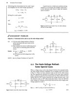
4.10 Use the mesh-current method to find the power
dissipated in the 2 ft resistor in the circuit shown.
30 V
Answer: 72 W.
4.11 Use the mesh-current method to find the mesh
current /
a
in the circuit shown.
75
VI
Answer: 15 A.
4.12 Use the mesh-current method to find the
power dissipated in the 1 ft resistor in the cir-
cuit shown.
16
A
^vw 4 Wv 4
10
A
e
20
'a
<\t,
15 n
in
•A^V-
2V*
2A

e
iovT*j
2
a
Answer: 36 W.
NOTE: Also try Chapter Problems 4.42, 4.44, 4.48, and 4.51.
6V
4,8 The Node-Voltage Method Versus
the Mesh-Current Method
The greatest advantage of both the node-voltage and mesh-current meth-
ods is that they reduce the number of simultaneous equations that must be
manipulated. They also require the analyst to be quite systematic in terms
of organizing and writing these equations. It is natural to ask, then, "When
is the node-voltage method preferred to the mesh-current method and
vice versa?" As you might suspect, there is no clear-cut answer. Asking a
number of questions, however, may help you identify the more efficient
method before plunging into the solution process:
• Does one of the methods result in fewer simultaneous equations
to solve?
• Does the circuit contain supernodes? If so, using the node-voltage
method will permit you to reduce the number of equations to
be solved.
4.8 The Node-Voltage Method Versus the Mesh-Current Method 107
• Does the circuit contain supermeshes? If so, using the mesh-current
method will permit you to reduce the number of equations to
be solved.
• Will solving some portion of the circuit give the requested solution?
If so, which method is most efficient for solving just the pertinent
portion of the circuit?
Perhaps the most important observation is that, for any situation, some

time spent thinking about the problem in relation to the various analytical
approaches available is time well spent. Examples 4.6 and 4.7 illustrate the
process of deciding between the node-voltage and mesh-current methods.
Example 4.6
Understanding the Node-Voltage Method Versus Mesh-Current Method
Find the power dissipated in the 300
Ct
resistor in
the circuit shown in Fig. 4.29.
300 ft J
1
-
-Wv
150 ft 100ft
-AAA^
250 ft
-AVv t
50 /
A
500 ft
256 V £200 ft
400 ft k
128
V
Figure 4.29 A The circuit for Example 4.6.
Solution
To find the power dissipated in the 300 H resistor,
we need to find either the current in the resistor or
the voltage across it. The mesh-current method
yields the current in the resistor; this approach

requires solving five simultaneous mesh equations,
as depicted in Fig. 4.30. In writing the five equa-
tions,
we must include the constraint /
A
= — i
b
.
Before going further, let's also look at the circuit
in terms of the node-voltage method. Note that, once
we know the node voltages, we can calculate either
the current in the 300 il resistor or the voltage across
it. The circuit has four essential nodes, and therefore
only three node-voltage equations are required to
describe the circuit. Because of the dependent volt-
age source between two essential nodes, we have to
sum the currents at only two nodes. Hence the prob-
lem is reduced to writing two node-voltage equations
and a constraint equation. Because the node-voltage
method requires only three simultaneous equations,
it is the more attractive approach.
Once the decision to use the node-voltage
method has been made, the next step is to select a
reference node. Two essential nodes in the circuit in
Fig. 4.29 merit consideration. The first is the refer-
ence node in
Fig.
4.31.
If this node is selected, one of
the unknown node voltages is the voltage across the

300
CL
resistor, namely, v
2
in Fig. 4.31. Once we
know this voltage, we calculate the power in the
300 f! resistor by using the expression
Psaon = «1/300.
300 ft -*'
A
-AAA.
150ft
100ft 250 ft
-AAA-—f—-WV-
500 ft
: f20uftSO
50
*A)f
.+.
Figure 4.30 A The circuit shown in Fig. 4.29, with the five
mesh currents.
300 ft J
s
vvV
150 ft
<^
500 ft
400 ft £ 128 V
Figure 4.31 A The circuit shown in Fig. 4.29, with a
reference node.

Note that, in addition to selecting the reference
node, we defined the three node voltages V\, v
2
, and
u
3
and indicated that nodes 1 and 3 form a super-
node, because they are connected by a dependent
voltage source. It is understood that a node voltage is
a rise from the reference node; therefore, in
Fig.
4.31,
we have not placed the node voltage polarity refer-
ences on the circuit diagram.
108 Techniques of Circuit Analysis
The second node that merits consideration as
the reference node is the lower node in the circuit,
as shown in Fig. 4.32. It is attractive because it has
the most branches connected to it, and the node-
voltage equations are thus easier to write. However,
to find either the current in the 300
11
resistor or
the voltage across it requires an additional calcula-
tion once we know the node voltages v
a
and v
c
. For
example, the current in the 300 H resistor is

(v
c
- v
a
)/300, whereas the voltage across the resis-
tor is v
r
- v».
300 ft
l*
128
V
Figure 4.32 A
The
circuit
shown
in
Fig.
4.29 with an
alternative reference node.
t?
3
+ 256
+ — = 0.
150
Att?
2
,
v
2

v
2
- Vi v
2
-
VT.
VI + 128 -
v-x
' + _•_ + + — — = 0.
300 250
400 500
From the supernode, the constraint equation is
v
2
v
3
= vi - 50/
A
= v, - —
Set 2 (Fig 4.32)
At%,
v
a
v
a
- 256 v.
d
- v
b
v

a
- v
c
_
200 150
Atv
c
,
100
300
We compare these two possible reference nodes
by means of the following sets of equations. The first
set pertains to the circuit shown in Fig.
4.31,
and the
second set is based on the circuit shown in
Fig.
4.32.
Set 1 (Fig 4.31)
At the supernode,
V\ V\ — v
2
v
3
V3 — v
2
v
3
— (v
2

+ 128)
KX)
+
250
+
200
+
400 500
v
c
v
c
+ 128 v
c
—
v
b
v
c
- v
a
400 500 250 300
From the supernode, the constraint equation is
50(v
c
- v
a
) v
c
- v

a
v
b
= 50/
A
300
You should verify that the solution of either set
leads to a power calculation of 16.57 W dissipated in
the 300
O,
resistor.
Example 4.7
Companng the Node-Voltage and Mesh-Current Methods
Find the voltage v
0
in the circuit shown in
Fig.
4.33.
Solution
At first glance, the node-voltage method looks
appealing, because we may define the unknown
voltage as a node voltage by choosing the lower ter-
minal of the dependent current source as the refer-
ence node. The circuit has four essential nodes and
two voltage-controlled dependent sources, so the
node-voltage method requires manipulation of
three node-voltage equations and two constraint
equations.
Let's now turn to the mesh-current method for
finding v

0
. The circuit contains three meshes, and
we can use the leftmost one to calculate v
0
. If we
let /
a
denote the leftmost mesh current, then
v
0
= 193
—
10/'
a
.
The presence of the two current
sources reduces the problem to manipulating a sin-
gle supermesh equation and two constraint equa-
tions.
Hence the mesh-current method is the more
attractive technique here.
4ft
0.8¾
6 ft 7.5 ft 8ft
Figure 4.33 •
The
circuit for Example 4.7.
4.9 Source Transformations
109
411 2.512

193
VI
r
~
-
"A
,,
W
AC
)^D^
-AMr-
-VvV
-Wr
6
n
7.5
n
8
a
Figure 4.34
A
The
circuit
shown
in
Fig.
4.33 with the three mesh currents.
4
0
2.5

ft *« 2 ft
-'vw
f -vw-
Ml93V^/t>0.4^ (T)o.5A
60
V^/v
and
the
constraint equations
are
i\j
—
/
a
=
0.4i;
A
=
0.8/
c
;
v
9
=
—
7.5/
b
;
and
/

c
—
/
b
= 0.5.
We
use the
constraint equations
to
write
the
super-
mesh equation
in
terms
of /
a
:
160
=
80*'
a
,
or /
a
= 2 A,
v
a
= 193 - 20 =
173

V.
The node-voltage equations
are
0.8
v
(l
7.5
ft "h
Figure
4.35
A
The
circuit
shown
in
Fig.
4.33 with
node
voltages.
To help
you
compare
the two
approaches,
we
summarize both methods.The mesh-current equa-
tions
are
based
on the

circuit shown
in Fig. 4.34,
and
the
node-voltage equations
are
based
on
the circuit shown
in Fig. 4.35. The
supermesh
equation
is
193
= 104 +
10
'b + 10/'c +
0.8v
0
,
v„
- 193
10
A
2.5
0.
2.5
10
^
b

t
0
5
1
% +
°'
8Ve
~
Va
~ 0
7.5
" 10
The constraint equations
are
v
9
= -v
b
, v
A
=
"«
a
- (v
b
+
0.8¾¾)
1
10
2.

We
use the
constraint equations
to
reduce
the
node-
voltage equations
to
three simultaneous equations
involving
v
()
, u
a
, and v
b
. You
should verify that
the
node-voltage approach also gives
v
0
=
173
V.
^ASSESSMENT PROBLEMS
Objective 3—Deciding between
the
node-voltage

and
mesh-current methods
4.13 Find
the
power delivered
by the
2
A
current
source
in the
circuit shown.
4.14 Find
the
power delivered
by the 4 A
current
source
in the
circuit shown.
4A
20 V
128 V
Answer: 70
W
NOTE: Also
try
Chapter Problems 4.52
and
4.53.

Answer: 40 W.
4.9 Source Transformations
Even though
the
node-voltage
and
mesh-current methods
are
powerful tech-
niques
for
solving circuits, we
are
still interested
in
methods that
can be
used
to simplify circuits. Series-parallel reductions
and
A-to-Y transformations
are
110 Techniques
of
Circuit Analysis
-•a
-•b
(b)
Figure 4.36 A Source transformations.
already on our list of simplifying techniques. We begin expanding this list

with source transformations. A source transformation, shown in Fig. 4.36,
allows a voltage source in series with a resistor to be replaced by a current
source in parallel with the same resistor or vice versa. The double-headed
arrow emphasizes that a source transformation is bilateral; that is, we can
start with either configuration and derive the other.
We need to find the relationship between v
s
and i
s
that guarantees the
two configurations in Fig. 4.36 are equivalent with respect to nodes a,b.
Equivalence is achieved if any resistor R
L
experiences the same current
flow, and thus the same voltage drop, whether connected between nodes
a,b in Fig. 4.36(a) or Fig. 4.36(b).
Suppose R
f
is connected between nodes a,b in Fig. 4.36(a). Using
Ohm's law, the current in R
L
is
tL
(4.52)
R + R
L
Now suppose the same resistor R
L
is connected between nodes a,b in
Fig. 4.36(b). Using current division, the current in R, is

R
'/.
(4.53)
if the two circuits in Fig. 4.36 are equivalent, these resistor currents must be
the same. Equating the right-hand sides of
Eqs.
4.52 and 4.53 and simplifying.
(4.54)
When Eq. 4.54 is satisfied for the circuits in Fig. 4.36, the current in R
L
is
the same for both circuits in the figure for all values of R
L
. If the current
through R
L
is the same in both circuits, then the voltage drop across R
{
is
the same in both circuits, and the circuits are equivalent at nodes a,b.
If the polarity of v
s
is reversed, the orientation of i
s
must be reversed
to maintain equivalence.
Example 4.8 illustrates the usefulness of making source transforma-
tions to simplify a circuit-analysis problem.
Example 4.8
Using Source Transformations to Solve a Circuit

a) For the circuit shown in Fig. 4.37, find the power
associated with the 6 V source.
b) State whether the 6 V source is absorbing or
delivering the power calculated in (a).
Solution
a) If we study the circuit shown in Fig. 4.37, know-
ing that the power associated with the 6 V
source is of interest, several approaches come
to mind. The circuit has four essential nodes
and six essential branches where the current is
unknown. Thus we can find the current in the
branch containing the 6 V source by solving
either three [6-(4-1)] mesh-current equa-
tions or three [4-1] node-voltage equations.
Choosing the mesh-current approach involves
6
V §30 n ?20£l
40
V
Figure 4.37 • The circuit for Example 4.8.
solving for the mesh current that corresponds
to the branch current in the 6 V source.
Choosing the node-voltage approach involves
solving for the voltage across the 30 O resistor,
from which the branch current in the 6 V
source can be calculated. But by focusing on
just one branch current, we can first simplify
the circuit by using source transformations.
4.9 Source Transformations 111
We must reduce the circuit in a way that pre-

serves the identity of the branch containing the 6 V
source. We have no reason to preserve the identity of
the branch containing the 40 V source. Beginning with
this branch, we can transform the 40 V source in
series with the 5 ft resistor into an 8 A current
source in parallel with a5fi resistor, as shown
in Fig. 4.38(a).
4 n
6
ii
-f 'WV
32 V
(a) First step
4
11
(b) Second step
412
12
O
19.2 V
(c) Third step
Figure 4.38 A Step-by-step simplification of the circuit
shown
in
Fig.
4.37.
Next, we can replace the parallel combination of
the 20 ft and 5 ft resistors with a 4 ft resistor.
This 4 ft resistor is in parallel with the 8 A source
and therefore can be replaced with a 32 V source

in series with a 4 ft resistor, as shown in
Fig. 4.38(b).The 32 V source is in series with 20 ft
of resistance and, hence, can be replaced by a cur-
rent source of 1.6 A in parallel with 20 ft, as shown
in Fig. 4.38(c). The 20 ft and 30 ft parallel resis-
tors can be reduced to a single 12 ft resistor. The
parallel combination of the 1.6 A current source
(d) Fourth step
and the 12 ft resistor transforms into a voltage
source of
19.2
V in series with 12 ft. Figure 4.38(d)
shows the result of this last transformation. The
current in the direction of the voltage drop across
the 6 V source is (19.2 - 6)/16, or 0.825 A.
Therefore the power associated with the 6 V
source is
p
6V
= (0.825)(6) = 4.95 W.
b) The voltage source is absorbing power.
A question that arises from use of the source transformation depicted
in Fig. 4.38
is,
"What happens if there is a resistance R
p
in parallel with the
voltage source or a resistance R
s
in series with the current source?" In

both cases, the resistance has no effect on the equivalent circuit that pre-
dicts behavior with respect to terminals a,b. Figure 4.39 summarizes this
observation.
The two circuits depicted in Fig. 4.39(a) are equivalent with respect to
terminals a,b because they produce the same voltage and current in any
resistor R
L
inserted between nodes a,b. The same can be said for the cir-
cuits in Fig. 4.39(b). Example 4.9 illustrates an application of the equiva-
lent circuits depicted in Fig. 4.39.
R
-wv—»a
»« \R,
-•b
(a)
(b)
Figure 4.39 • Equivalent circuits containing a
resistance in parallel with a voltage source or in series
with a current source.
112 Techniques of Circuit Analysis
Example 4.9
Using Special Source Transformation Techniques
a) Use source transformations to find the voltage
v
()
in the circuit shown in Fig. 4.40.
b) Find the power developed by the 250 V voltage
source.
c) Find the power developed by the 8 A current
source.

b) The current supplied by the 250 V source equals the
current in the 125
ft
resistor plus the current in the
25
ft
resistor. Thus
250 250
-
20
„ „
'<
=
l25
+
-^-
=1UA
-
25
ft
250
V
Figure 4.40 A The circuit for Example 4.9.
Solution
Therefore the power developed by the voltage source is
/>
25()
v(developed)
=
(250)(11.2) = 2800 W.

c) To find the power developed by the 8 A current source,
we first find the voltage across the source. If we let v
s
represent the voltage across the source, positive at the
upper terminal of the source, we obtain
a) We begin by removing the 125
ft
and 10
ft
resis-
tors,
because the 125
ft
resistor is connected across
the 250 V voltage source and the 10
ft
resistor is
connected in series with the 8 A current source. We
also combine the series-connected resistors into
a
single resistance of 20
ft.
Figure 4.41 shows the sim-
plified circuit.
v
s
+ 8(10) = v
0
= 20,
or v

s
= -60 V,
and the power developed by the 8 A source is 480 W.
Note that the 125
ft
and 10
ft
resistors do not affect
the value of v
0
but do affect the power calculations.
25
ft
250 V
Figure 4.41
•
A
simplified version of the circuit shown in Fig. 4.40.
Figure 4.42
•
The circuit shown in Fig. 4.41 after
a
source
transformation.
We now use a source transformation to replace
the 250 V source and 25
ft
resistor with
a
10

A
source in parallel with the 25
ft
resistor, as shown in
Fig. 4.42. We can now simplify the circuit shown in
Fig. 4.42 by using Kirchhoffs current law to com-
bine the parallel current sources into
a
single
source. The parallel resistors combine into
a
single
resistor. Figure 4.43 shows
the
result. Hence
v„ = 20 V.
+
D„5
io
ft
Figure 4.43 A The circuit shown in Fig. 4.42 after combining
sources and resistors.
4.10 Thevenin and Norton Equivalents 113
/"ASSESSMENT PROBLEM
Objective 4—Understand source transformation
4.15 a) Use a series of source transformations to
find the voltage v in the circuit shown.
b) How much power does the 120 V source
deliver to the circuit?
Answer: (a) 48 V;

(b) 374.4 W.
NOTE: Also try Chapter Problems 4.59 and 4.60.
20
a ,
j
60V
-r
(t
)
36A
1120 V
L
1.6 a
4.10 Thevenin and Norton Equivalents
At times in circuit analysis, we want to concentrate on what happens at
a specific pair of terminals. For example, when we plug a toaster into an
outlet, we are interested primarily in the voltage and current at the ter-
minals of the toaster. We have little or no interest in the effect that con-
necting the toaster has on voltages or currents elsewhere in the circuit
supplying the outlet. We can expand this interest in terminal behavior
to a set of appliances, each requiring a different amount of power.
We then are interested in how the voltage and current delivered at the
outlet change as we change appliances. In other words, we want to focus
on the behavior of the circuit supplying the outlet, but only at the out-
let terminals.
Thevenin and Norton equivalents are circuit simplification techniques
that focus on terminal behavior and thus are extremely valuable aids in
analysis. Although here we discuss them as they pertain to resistive cir-
cuits,
Thevenin and Norton equivalent circuits may be used to represent

any circuit made up of linear elements.
We can best describe a Thevenin equivalent circuit by reference to
Fig. 4.44, which represents any circuit made up of sources (both inde-
pendent and dependent) and resistors. The letters a and b denote the
pair of terminals of interest. Figure 4.44(b) shows the Thevenin equiva-
lent. Thus, a Thevenin equivalent circuit is an independent voltage
source V
Th
in series with a resistor R
Th
, which replaces an interconnec-
tion of sources and resistors. This series combination of V
Th
and R
T
h is
equivalent to the original circuit in the sense that, if we connect the
same load across the terminals a,b of each circuit, we get the same volt-
age and current at the terminals of the load. This equivalence holds for
all possible values of load resistance.
To represent the original circuit by its Thevenin equivalent, we must
be able to determine the Thevenin voltage V
Jh
and the Thevenin resist-
ance R
lh
. First, we note that if the load resistance is infinitely large, we
have an open-circuit condition. The open-circuit voltage at the terminals
a,b in the circuit shown in Fig. 4.44(b) is Vj
h

. By hypothesis, this must be
• a
A resistive
network containing
independent and
dependent sources
(a)
(b)
Figure 4.44 A (a) A general circuit, (b) The Thevenin
equivalent circuit.
114 Techniques of Circuit Analysis
the same as the open-circuit voltage at the terminals a,b in the original
circuit. Therefore, to calculate the Thevenin voltage V
Th
, we simply calcu-
late the open-circuit voltage in the original circuit.
Reducing the load resistance to zero gives us a short-circuit condition.
If we place a short circuit across the terminals a,b of the Thevenin equiva-
lent circuit, the short-circuit current directed from a to b is
/„-
=
Tli
Th
(4.55)
By hypothesis, this short-circuit current must be identical to the short-circuit
current that exists in a short circuit placed across the terminals a,b of the
original network. From Eq. 4.55,
R
Th
-

V-,
ih
(4.56)
Thus the Thevenin resistance is the ratio of the open-circuit voltage to the
short-circuit current.
40
^vw—• a
+ +
2sy
Cz)
2
°^f
3A
0
)
V]
^
Finding a Thevenin Equivalent
To find the Tlievenin equivalent of the circuit shown in Fig. 4.45, we first
calculate the open-circuit voltage of
v.
db
.
Note that when the terminals a,b
are open, there is no current in the 4 O resistor. Therefore the open-circuit
voltage
v.
db
is identical to the voltage across the
3

A current source, labeled
V\. We find the voltage by solving a single node-voltage equation.
Choosing the lower node as the reference node, we get
Figure 4.45 • A circuit used to illustrate a Thevenin
equivalent.
Vi - 25 V]
— + — - 3 = 0.
5 20
(4.57)
Solving for V\ yields
v
x
= 32 V.
(4.58)
25 V
Figure 4.46 • The circuit shown in Fig. 4.45 with
terminals a and b short-circuited.
Hence the Thevenin voltage for the circuit is 32 V.
The next step is to place a short circuit across the terminals and calcu-
late the resulting short-circuit current. Figure 4.46 shows the circuit with
the short in place. Note that the short-circuit current is in the direction of
the open-circuit voltage drop across the terminals a,b. If the short-circuit
current is in the direction of the open-circuit voltage rise across the termi-
nals,
a minus sign must be inserted in Eq. 4.56.
The short-circuit current (/
sc
) is found easily once v
2
is known. Therefore

the problem reduces to finding v
2
with the short in place. Again, if we use the
lower node as the reference node, the equation for v
2
becomes
v
2
- 25 ih v-y
(4.59)
4.10 Thevenin
and
Norton Equivalents
115
Solving
Eq. 4.59 for v
2
gives
th
= 16 V.
(4.60)
Hence,
the
short-circuit current
is
16
A A
<ac
=
"J"

=
4 A
-
(4.61)
We
now
find the Thevenin resistance
by
substituting
the
numerical results
from Eqs. 4.58
and
4.61 into Eq. 4.56:
R
Th
=
V
Th
32
4
8H.
(4.62)
Figure 4.47 shows the Thevenin equivalent
for the
circuit shown
in
Fig.
4.45.
You should verify that,

if a 24
Cl
resistor
is
connected across
the
ter-
minals
a,b in Fig.
4.45,
the
voltage across
the
resistor will
be 24 V and
the current
in the
resistor will
be 1 A, as
would
be the
case with
the
Thevenin circuit
in
Fig. 4.47. This same equivalence between
the
circuit
in Figs.
4.45 and 4.47

holds
for any
resistor value connected between
nodes
a.b.
The Norton Equivalent
A Norton equivalent circuit consists
of an
independent current source
in parallel with
the
Norton equivalent resistance, We
can
derive
it
from
a Thevenin equivalent circuit simply
by
making
a
source transforma-
tion. Thus
the
Norton current equals
the
short-circuit current
at the
terminals
of
interest,

and the
Norton resistance
is
identical
to the
Thevenin resistance.
32
V
SO
'VW
• a
Figure
4.47 •
The Thevenin equivalent of the circuit
shown
in
Fig. 4.45.
4
O
-wv—•
a
J25V J20I1
( f J3A
-•b
Step
1:
Source transformation
t
Step
2:

Parallel sources
and
parallel resistors combined
•
4ft
•—-Wv—e
a
8A
4
0
-•b
Step
3:
Source transformation; series
resistors combined, producing
the Thevenin equivalent circuit
8ft
-VW-
32 V
Using Source Transformations
Sometimes
we can
make effective
use of
source transformations
to
derive
a
Thevenin
or

Norton equivalent circuit.
For
example,
we can
derive
the
Thevenin
and
Norton equivalents
of the
circuit shown
in
Fig. 4.45 by
making
the
series
of
source transformations shown
in
Fig. 4.48. This technique
is
most useful when
the
network contains only
independent sources.
The
presence
of
dependent sources requires
retaining

the
identity
of the
controlling voltages and/or currents,
and
this constraint usually prohibits continued reduction
of the
circuit
by source transformations.
We
discuss
the
problem
of
finding
the
Thevenin equivalent when
a
circuit contains dependent sources
in
Example
4.10.
Step
4:
Source transformation, producing
the Norton equivalent circuit
4A
8
O
Figure

4.48 •
Step-by-step derivation
of
the Thevenin
and Norton equivalents
of
the circuit shown
in
Fig. 4.45.