Electric Circuits, 9th Edition P15 docx

116 Techniques of Circuit Analysis
Example 4.10
Finding the Thevenin Equivalent of a Circuit with a Dependent Source
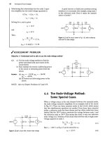
Find the Thevenin equivalent for the circuit con-
taining dependent sources shown in Fig. 4.49.
2kO
5V
Figure 4.49 • A circuit used to illustrate a Thevenin equivalent
when the circuit contains dependent sources.
Figure 4.50 • The circuit shown in Fig. 4.49 with terminals a
and b short-circuited.
Solution
The first step in analyzing the circuit in Fig. 4.49 is
to recognize that the current labeled i
x
must be
zero.
(Note the absence of a return path for i
x
to
enter the left-hand portion of the circuit.) The
open-circuit, or Thevenin, voltage will be the volt-
age across the 25 ft resistor. With i
x
= 0,
^Th = ^ab = (-200(25) = -500/.
The current
/'
is
3v 3V
i =

Th
2000 2000
In writing the equation for i, we recognize that the
Thevenin voltage is identical to the control voltage.
When we combine these two equations, we obtain
V
Th
-5 V.
To calculate the short-circuit current, we place
a short circuit across a,b. When the terminals a,b are
shorted together, the control voltage v is reduced to
zero.
Therefore, with the short in place, the circuit
shown in Fig. 4.49 becomes the one shown in
Fig. 4.50. With the short circuit shunting the 25 ft
resistor, all the current from the dependent current
source appears in the short, so
20/.
As the voltage controlling the dependent volt-
age source has been reduced to zero, the current
controlling the dependent current source is
2.5 mA.
2000
Combining these two equations yields a short-circuit
current of
i
sc
= -20(2.5) = -50 mA.
From /
sc

and V
Th
we get
R
Th
-
V
l'h
-5
'Ur -50
X 10-
1
= 100 ft.
Figure 4.51 illustrates the Thevenin equivalent
for the circuit shown in Fig. 4.49. Note that the
ref-
erence polarity marks on the Thevenin voltage
source in Fig. 4.51 agree with the preceding equa-
tion for V
Th
.
100 ft
5V
Figure 4.51 • The Thevenin equivalent for the circuit shown in
Fig.
4.49.
4.11 More on Deriving a Thevenin Equivalent 117
^ASSESSMENT PROBLEMS
Objective 5—Understand Thevenin and Norton equivalents
4.16 Find the Thevenin equivalent circuit with respect

to the terminals a,b for the circuit shown.
Answer: V
ah
= V
T
u = 64.8 V^
T
h = 6a
Th
72
VI
12
n
50
8fl
:20il
4.17 Find the Norton equivalent circuit with respect
to the terminals a,b for the circuit shown.
Answer: /
N
= 6 A (directed toward a), i?
N
= 7.5 ft.
4.18 A voltmeter with an internal resistance of
100 kft is used to measure the voltage v
AB
in the
circuit shown. What is the voltmeter reading?
Answer: 120 V.
NOTE: Also try Chapter Problems 4.63, 4.64, and 4.71.

36 V
6
12
kO
15
kH
VW • A
f J18mA | 60 kft
y,\n
-•B
4.11 More on Deriving a Thevenin
Equivalent
The technique for determining JR
Th
that we discussed and illustrated in
Section 4.10 is not always the easiest method available. Two other meth-
ods generally are simpler to use. The first is useful if the network contains
only independent sources. To calculate R
Th
for such a network, we first
deactivate all independent sources and then calculate the resistance seen
looking into the network at the designated terminal pair. A voltage source
is deactivated by replacing it with a short circuit. A current source is deac-
tivated by replacing it with an open circuit. For example, consider the cir-
cuit shown in Fig. 4.52. Deactivating the independent sources simplifies
the circuit to the one shown in Fig.
4.53.
The resistance seen looking into
the terminals a,b is denoted
i?

al
,,
which consists of the 4 ft resistor in series
with the parallel combinations of the 5 and 20 ft resistors.Thus,
Kab = R
Th
4 +
5 x 20
25
8 ft. (4.63)
Note that the derivation of R
Th
with Eq. 4.63 is much simpler than the
same derivation with Eqs. 4.57-4.62.
25 V
Figure 4.52 •
A
circuit used to illustrate a Thevenin
equivalent.
5^
R
ab
Figure 4.53 • The circuit shown in Fig. 4.52 after deac-
tivation of the independent sources.
118 Techniques of Circuit Analysis
If the circuit or network contains dependent sources, an alternative
procedure for finding the Thevenin resistance R
Th
is as follows. We first
deactivate all independent sources, and we then apply either a test voltage

source or a test current source to the Thevenin terminals a,b.The Thevenin
resistance equals the ratio of the voltage across the test source to the cur-
rent delivered by the test source. Example 4.11 illustrates this alternative
procedure for finding R
Th
, using the same circuit as Example 4.10.
Example
4.11 Finding the Thevenin Equivalent Using a Test Source
Find the Thevenin resistance R
Th
for the circuit in
Fig. 4.49, using the alternative method described.
Solution
We first deactivate the independent voltage source
from the circuit and then excite the circuit from the
terminals a,b with either a test voltage source or a
test current source. If we apply a test voltage source,
we will know the voltage of the dependent voltage
source and hence the controlling current
i.
Therefore
we opt for the test voltage source. Figure 4.54 shows
the circuit for computing the Thevenin resistance.
2kH
'/•
20/
f
25
0 v
T

Figure 4.54 • An alternative method for computing the
Thevenin resistance.
The externally applied test voltage source is
denoted v
r
, and the current that it delivers to the
circuit is labeled i
T
. To find the Thevenin resistance,
we simply solve the circuit shown in Fig. 4.54 for the
ratio of the voltage to the current at the test source;
that is, R
Th
= Vrjij. From Fig. 4.54,
(4.64)
(4.65)
We then substitute Eq. 4.65 into Eq. 4.64 and solve
the resulting equation for the ratio v
T
/i
r
:
v
r
b\)v
T
lT
~ 25 2000'
/'-/• 1 6 50
v

T
25 200 5000
From Eqs. 4.66 and 4.67,
#Th = — = 100 H.
i
r
1
100*
(4.66)
(4.67)
(4.68)
Figure 4.55 A The application of
a
Thevenin equivalent
in circuit analysis.
In general, these computations are easier than those involved in com-
puting the short-circuit current. Moreover, in a network containing only
resistors and dependent sources, you must use the alternative method,
because the ratio of the Thevenin voltage to the short-circuit current is
indeterminate. That
is,
it is the ratio 0/0.
Using the Thevenin Equivalent in the Amplifier Circuit
At times we can use a Thevenin equivalent to reduce one portion of a cir-
cuit to greatly simplify analysis of the larger network. Let's return to the
circuit first introduced in Section 2.5 and subsequently analyzed in
Sections 4.4 and
4.7.
To aid our discussion, we redrew the circuit and iden-
tified the branch currents of interest, as shown in Fig. 4.55.

As our previous analysis has shown, i
B
is the key to finding the other
branch currents. We redraw the circuit as shown in Fig. 4.56 to prepare to
replace the subcircuit to the left of V
{)
with its Thevenin equivalent. You
4.11 More on Deriving a Thevenin Equivalent 119
Figure 4.56 • A modified version of the circuit shown
in
Fig.
4.55.
Figure 4.57 • The circuit shown in Fig. 4.56 modified
by a Thevenin equivalent.
should be able to determine that this modification has no effect on the
branch currents i[, ij, hh
an
d /#.
Now we replace the circuit made up of V
cc
, i?x, and R
2
with a
Thevenin equivalent, with respect to the terminals b.d.The Thevenin volt-
age and resistance are
V
l'h
R
rh
R^R

2
R
Y
+ R
2
(4.69)
(4.70)
With the Thevenin equivalent, the circuit in Fig. 4.56 becomes the one
shown in Fig. 4.57.
We now derive an equation for /'# simply by summing the voltages
around the left mesh. In writing this mesh equation, we recognize that
i
E
= (1 + p)i
B
- Thus,
^TK
= R-ntB + V
Q
+ R
E
(1 + p)i
B
,
(4.71)
from which
h =
v
Th
- v

{
R
Th
+ (1+ fi)R
E
(4.72)
When we substitute Eqs. 4.69 and 4.70 into Eq. 4.72, we get the same
expression obtained in Eq.2.25. Note that when we have incorporated the
Thevenin equivalent into the original circuit, we can obtain the solution
for i
B
by writing a single equation.
^ASSESSMENT PROBLEMS
Objective 5—Understand Thevenin and Norton equivalents
4.19 Find the Thevenin equivalent circuit with respect
to the terminals a,b for the circuit shown.
Answer: V
Th
= v
ab
= 8 V, R
Th
= 10.
4.20 Find the Thevenin equivalent circuit with
respect to the terminals a,b for the circuit
shown. (Hint: Define the voltage at the left-
most node as v, and write two nodal equations
with V
Th
as the right node voltage.)

24 V
J l
x
2H
—Wv—
4A(T)
i.'Asn
-•b
Answer:
F
Tll
- v
ah
= 30 V, R
Th
= 10 0,.
20
n
160/
^
60aj4A( I
so
ft
f
40
a
f
i
is
-•b

NOTE: Also try Chapter Problems 4.74 and 4.77.
120 Techniques of Circuit Analysis
Resistive network
containing
independent and
dependent sources
b«—
RL
Figure 4.58 • A circuit describing maximum power
transfer.
R,
Figure 4.59 • A circuit used to determine the value of
R
L
for maximum power transfer.
4,12 Maximum Power Transfer
Circuit analysis plays an important role in the analysis of systems designed
to transfer power from a source to a load. We discuss power transfer in
terms of two basic types of systems. The first emphasizes the efficiency of
the power transfer. Power utility systems are a good example of this type
because they are concerned with the generation, transmission, and distri-
bution of large quantities of electric power. If a power utility system is
inefficient, a large percentage of the power generated is lost in the trans-
mission and distribution processes, and thus wasted.
The second basic type of system emphasizes the amount of power trans-
ferred. Communication and instrumentation systems are good examples
because in the transmission of information, or data, via electric signals, the
power available at the transmitter or detector is limited.
Thus,
transmitting as

much of this power as possible to the receiver, or load, is desirable. In such
applications the amount of power being transferred is small, so the efficiency
of transfer is not a primary concern. We now consider maximum power
transfer in systems that can be modeled by a purely resistive circuit.
Maximum power transfer can best be described with the aid of the cir-
cuit shown in Fig.
4.58.
We assume a resistive network containing independ-
ent and dependent sources and a designated pair of terminals, a,b, to which a
load, R
L
, is to be connected.The problem is to determine the value of R
L
that
permits maximum power delivery to R
L
. The first step in this process is to
recognize that a resistive network can always be replaced by its Thevenin
equivalent. Therefore, we redraw the circuit shown in Fig. 4.58 as the one
shown in
Fig.
4.59.
Replacing the original network by
its
Thevenin equivalent
greatly simplifies the task of finding R
L
. Derivation of R
L
requires express-

ing the power dissipated in R
L
as a function of the three circuit parameters
V
Th
,
i?
Th
,
and R
L
. Thus
p = i
2
R
L
V
Th
Rjh + ^L
Ri,
(4.73)
Next, we recognize that for a given circuit, Vj^ and R
Th
will be fixed.
Therefore the power dissipated is a function of the single variable R
L
, To
find the value of R
L
that maximizes the power, we use elementary calculus.

We begin by writing an equation for the derivative of p with respect to R
L
:
dp
~d~R~,
V
2
Th
(R
Th
+ R
L
)
2
- R
L
-2(R
Th
+ R
L
)
(ftn, + R
L
)
4
The derivative is zero and p is maximized when
(R
Th
+ R
L

)
2
= 2R
L
(Rru + RL)-
(4.74)
(4.75)
Solving Eq. 4.75 yields
Condition for maximum power transfer •
R,
R
Th-
(4.76)
Thus maximum power transfer occurs when the load resistance R
L
equals
the Thevenin resistance R
Th
. To find the maximum power delivered to R
L
,
we simply substitute Eq. 4.76 into Eq. 4.73:
^fh^L
V
2
Th
(4.77)
"
ndX
{2R

L
f AR
L
The analysis of a circuit when the load resistor is adjusted for maximum
power transfer is illustrated in Example 4.12.
4.12 Maximum
Power
Transfer 121
Example 4.12 Calculating the Condition for Maximum Power Transfer
a) For the circuit shown in Fig. 4.60, find the value
of R
f
that results in maximum power being
transferred to R
L
.
360 V
300 V
25 0
:R,
Figure 4.61 A Reduction of the circuit shown in Fig. 4.60 by
means of a Thevenin equivalent.
Figure 4.60 •
The
circuit for Example 4.12.
b) The maximum power that can be delivered to
R
L
h
b) Calculate the maximum power that can be deliv-

ered to R
L
.
c) When R
f
is adjusted for maximum power trans-
fer, what percentage of the power delivered by
the 360 V source reaches
R
L
*>
/300V
/W = \j£) (25) = 900 W.
c) When R
L
equals 25 O, the voltage v
nb
is
Solution
a) The Thevenin voltage for the circuit to the left of
the terminals a,b is
lff)< •
From Fig. 4.60, when v
nb
equals 150 V, the cur-
rent in the voltage source in the direction of the
voltage rise across the source is
VTU
= y~(360) = 300 V.
. _ 360 - 150 _ 210 _

lj
" " 30 " 30
== ? A
-
The Thevenin resistance is
(150)(30)
J?™-
180
-25 a
Therefore, the source is delivering 2520 W to the
circuit, or
Ps = -4(360) = -2520 W.
Replacing the circuit to the left of the termi-
nals a,b with its Thevenin equivalent gives
us the circuit shown in Fig. 4.61, which indi-
cates that R
L
must equal 25 fl for maximum
power transfer.
The percentage of the source power delivered to
the load is
900
2520
X 100 =
35.71%.
122 Techniques of Circuit Analysis
/ASSESSMENT PROBLEMS
Objective 6—Know the condition for and calculate maximum power transfer to resistive load
4.21 a) Find the value of R that enables the circuit
shown to deliver maximum power to the

terminals a,b.
b) Find the maximum power delivered to R.
100
V
C-)
4.22 Assume that the circuit in Assessment
Problem 4.21 is delivering maximum power to
the load resistor R.
a) How much power is the 100 V source deliv-
ering to the network?
b) Repeat (a) for the dependent voltage
source.
c) What percentage of the total power gener-
ated by these two sources is delivered to the
load resistor /??
Answer:
Answer: (a) 3 0;
(b) 1.2 kW.
NOTE: Also try Chapter Problems 4.83 and 4.87.
(a) 3000 W;
(b)800W;
(c) 31.58%.
4.13 Superposition
A linear system obeys the principle of superposition, which states that
whenever a linear system is excited, or driven, by more than one inde-
pendent source of energy, the total response is the sum of the individual
responses. An individual response is the result of an independent source
acting alone. Because we are dealing with circuits made up of inter-
connected linear-circuit elements, we can apply the principle of superposi-
tion directly to the analysis of such circuits when they are driven by more

than one independent energy source. At present, we restrict the discussion
to simple resistive networks; however, the principle is applicable to any
linear system.
Superposition is applied in both the analysis and the design of circuits.
In analyzing a complex circuit with multiple independent voltage and cur-
rent sources, there are often fewer, simpler equations to solve when the
effects of the independent sources are considered one at a time. Applying
superposition can thus simplify circuit analysis. Be aware, though, that
sometimes applying superposition actually complicates the
analysis,
produc-
ing more equations to solve than with an alternative method. Superposition
is required only if the independent sources in a circuit are fundamentally
different. In these early chapters, all independent sources are dc sources, so
superposition is not required. We introduce superposition here in anticipa-
tion of later chapters in which circuits will require it.
Superposition is applied in design to synthesize a desired circuit
response that could not be achieved in a circuit with a single source. If the
desired circuit response can be written as a sum of two or more terms, the
response can be realized by including one independent source for each
term of the response. This approach to the design of circuits with complex
responses allows a designer to consider several simple designs instead of
one complex design.
4.13 Superposition 123
We demonstrate the superposition principle by using it to find the
branch currents in the circuit shown in Fig. 4.62. We begin by finding the
branch currents resulting from the 120 V voltage source. We denote those
currents with a prime. Replacing the ideal current source with an open cir-
cuit deactivates it; Fig. 4.63 shows this. The branch currents in this circuit
are the result of only the voltage source.

We can easily find the branch currents in the circuit in Fig. 4.63 once
we know the node voltage across the 3 ft resistor. Denoting this voltage
Vi, we write
from which
V\ - 120 Vt Vi
— + — + ——
6 3 2 + 4
v
]
= 30 V.
= 0,
(4.78)
120 V
12A
Figure 4.62 •
A
circuit
used
to illustrate superposition.
120 V
60,
'VW-
V]
20
:3ft
14
If 4XI
(4.79) Figure 4.63 •
The
circuit

shown
in
Fig.
4.62 with the
current source deactivated.
Now we can write the expressions for the branch currents i[
—
i'±
directly:
120 - 30
= 15 A,
*-?-
10 A,
(4.80)
(4.81)
«3
6
(4.82)
To find the component of the branch currents resulting from the current
source, we deactivate the ideal voltage source and solve the circuit shown in
Fig.
4.64.
The double-prime notation for the currents indicates they are the
components of the total current resulting from the ideal current source.
We determine the branch currents in the circuit shown in Fig. 4.64 by
first solving for the node voltages across the 3 and 4 ft resistors, respec-
tively. Figure 4.65 shows the two node voltages. The two node-voltage
equations that describe the circuit are
6ft
->vw

12A
Figure 4.64 •
The
circuit
shown
in
Fig.
4.62 with the
voltage source deactivated.
3 6 2
VA - V* VA
4
n
3
+ -Y + 12 = 0.
2 4
Solving Eqs. 4.83 and 4.84 for v
3
and i>
4
, we get
(4.83)
(4.84)
6H
-'WV
Figure 4.65 A
The
circuit
shown
in

Fig.
4.64 showing
the node voltages v
3
and v
4
.
^3
-12 V,
(4.85)
v
4
= -24 V.
(4.86)
Now we can write the branch currents /" through
i%
directly in terms of the
node voltages v
3
and v
4
:
*-?-?-".
(4.87)
124 Techniques of Circuit Analysis
«-?-^~4
A.
(4.88)
.„ v
3

~ v
4
-12 + 24
f
3 = —^
=
« = 6 A,
(4.89)
'4
«4
4
-24
= -6 A. (4.90)
To find the branch currents in the original circuit, that
is,
the currents
ij,
/
2
, /3, and i
4
in Fig. 4.62, we simply add the currents given by
Eqs.
4.87-4.90 to the currents given by
Eqs.
4.80-4.82:
h =
i'l
+ % = 15 + 2 = 17 A,
/

2
= /
2
+ i
2
' = 10 - 4 = 6 A,
«3 = '3 + /3=5 + 6= 11 A,
/
4
= /4 + /4 =
5-6=-1
A.
(4.91)
(4.92)
(4.93)
(4.94)
You should verify that the currents given by
Eqs.
4.91-4.94 are the correct
values for the branch currents in the circuit shown in
Fig.
4.62.
When applying superposition to linear circuits containing both independ-
ent and dependent sources, you must recognize that the dependent sources
are never deactivated. Example 4.13 illustrates the application of superposi-
tion when a circuit contains both dependent and independent sources.
Example 4.13 Using Superposition to Solve a Circuit
Use the principle of superposition to find v
()
in the

circuit shown in
Fig.
4.66.
0.4 v
A
10 V
^>
(-,,^20
n "A^lOft ( f )5 A
2 i
x
O
Figure 4.66 A The circuit for Example 4.13.
Solution
We begin by finding the component of v
0
resulting
from the
10
V source. Figure 4.67 shows the circuit.
With the 5 A source deactivated,
v'&
must equal
(-0.414)(10). Hence, v'
A
must be zero, the branch
containing the two dependent sources is open, and
20
10 V
v'o

= 25(10) = 8 V.
0.4 v
A
'
»</£20fi y
A
'|l0n
2/V
O
1
Figure 4.67 • The circuit shown in Fig. 4.66 with the 5 A
source deactivated.
When the 10 V source is deactivated, the circuit
reduces to the one shown in Fig. 4.68. We have
added a reference node and the node designations
a, b, and c to aid the discussion. Summing the cur-
rents away from node a yields
J} + y - OAvl = 0, or 5v» - 8v£ = 0.
Summing the currents away from node b gives
0.4^.^-5
0, or
4v% + v
b
- 2¾ = 50.
We now use
v
b
= 2il + vl
to find the value for v'i. Thus,
5vl = 50, or vl = 10 V.

Practical Perspective
125
From the node a equation,
5t>g = 80, or z?g = 16 V.
The value of v
a
is the sum of
v'
t)
and
v"„
or 24 V.
0.4 »
A
»
<e>rl
<'j2on v
A
"|ion
(t)
5A
2 4"
o
Figure
4.68 •
The circuit shown
in
Fig. 4.66 with
the
10 V

source deactivated.
NOTE: Assess your understanding of this material
by trying Chapter Problems 4.91 and 4.96.
Practical Perspective
Circuits with Realistic Resistors
It
is not
possible
to
fabricate identical electrical components.
For
example,
resistors produced from
the
same manufacturing process
can
vary
in
value
by
as
much
as
20%. Therefore,
in
creating
an
electrical system
the
designer

must consider
the
impact that component variation will have
on the
per-
formance
of the
system.
One way to
evaluate this impact
is by
performing
sensitivity analysis. Sensitivity analysis permits
the
designer
to
calculate
the impact
of
variations
in the
component values
on the
output
of
the sys-
tem.
We
will
see how

this information enables
a
designer
to
specify
an
acceptable component value tolerance
for
each
of
the system's components.
Consider the circuit shown
in
Fig. 4.69. To illustrate sensitivity analysis,
we will investigate the sensitivity
of
the node voltages
V\
and
v
2
to
changes
in
the
resistor
/^.
Using nodal analysis
we
can derive

the
expressions
for V\
and
v
2
as
functions
of
the circuit resistors
and
source currents.
The
results
are given
in
Eqs.
4.95 and 4.96:
Vi
v
2
=
(*! + R
2
)(R
3
+ R
4
) + R3R4
RsR^Ri + R

2
)l
s
i ~ Rilgi]
(*, + R
2
)(R
3
+ R
4
) +
R
3
R
4
'
(4.95)
(4.96)
The sensitivity
of V\
with respect
to Ri is
found
by
differentiating Eq.
4.95
with respect
to R
u
and

similarly
the
sensitivity
of v
2
with respect
to R^ is
found
by
differentiating Eq.
4.96
with respect
to R
l
.
We
get
dVx
[R3R4 + Ri(R3 + R
4
)}{R,R
4
I
g
2 ~ [R3R4 + fl
2
(*3 +
RA)]I
8
I}

dR\
~
[(/?!
+ R
2
)(R
3
+ R
4
) + R
3
R
4
Y
(4.97)