Electric Circuits, 9th Edition P22 potx

186 Inductance, Capacitance, and
Mutual
Inductance
(Note that 5 V is the voltage on the capacitor at
the end of the preceding interval.) Then,
v = (10*7 - 12.5 X 10¥ - 10) V,
p = t»,
= (62.5 X
10
12
/
3
- 7.5 x 10V + 2.5 X 10
5
/ - 2) W,
w = —Cv~,
2
0
V (V)
t(fis)
12 A 9*3 ^),2
= (15.625 X 10
u
r - 2.5 X l()r + 0.125 X 10
(
V
For/ > 40^ts,
- 2/ + 10~
3
) J.
v = 10 V,

p = vi = 0,
w = —Cv
2
= 10/xJ.
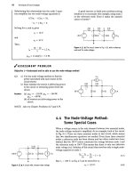
b) The excitation current and the resulting voltage,
power, and energy are plotted in Fig. 6.12.
c) Note that the power is always positive for the
duration of the current pulse, which means that
energy is continuously being stored in the capac-
itor. When the current returns to zero, the stored
energy is trapped because the ideal capacitor
offers no means for dissipating energy. Thus a
voltage remains on the capacitor after i returns
to zero.
10
5
0
—n
10
1
20
l
30
i
40
1
50
I
60
t((XS)

p(mw
500
400
300
200
100
0
)
^1
10
1
20
1
30
40
1
50
J
60
tips)
w(
10
8
6
4
2
0
nJ)
10
i

20
I
30
1
40
l
50
I
60
Figure 6.12 •
The
variables /', v, p, and to versus
Example 6.5.
t(fJ!S)
t for
^/ASSESSMENT PROBLEMS
Objective 2—Know and be able to use the equations for voltage, current, power, and energy in a capacitor
6.2
The voltage at the terminals of the 0.6 /xF
capacitor shown in the figure is 0 for t < 0 and
4Qe
-ism)t
sin
30,000/ V for t > 0. Find (a)
/'(0);
(b) the power delivered to the capacitor at
/ =
77-/8O
ms; and (c) the energy stored in the
capacitor at t = TT/80 ms.

0.6 ^F
NOTE: Also try Chapter Problems 6.16 and 6.17.
Answer: (a) 0.72 A;
(b) -649.2 mW;
(c) 126.13 AtJ.
6.3 The current in the capacitor of Assessment
Problem 6.2 is 0 for t < 0 and 3 cos 50,000/ A
for t a 0. Find (a) v{t)\ (b) the maximum power
delivered to the capacitor at any one instant of
time;
and (c) the maximum energy stored in the
capacitor at any one instant of time.
Answer: (a) 100 sin 50,000/ V, / > 0;
(b)150W;(c)3mJ.
6.3 Series-Parallel Combinations of
Inductance
and Capacitance 187
6.3 Series-Parallel Combinations
of Inductance and Capacitance
Just as series-parallel combinations of resistors can be reduced to a single
equivalent resistor, series-parallel combinations of inductors or capacitors
can be reduced to a single inductor or capacitor. Figure 6.13 shows induc-
tors in series. Here, the inductors are forced to carry the same current; thus
we define only one current for the series combination. The voltage drops
across the individual inductors are
Figure 6.13 A Inductors in series.
di di di
„ = £,-, v
2
= L

1Jt
, and v
}
= L,
The voltage across the series connection is
v = v\ + v
2
+ v
3
= (L
{
+ L
2
+ L?)—
at
from which it should be apparent that the equivalent inductance of series-
connected inductors is the sum of the individual inductances. For n induc-
tors in series,
L
eQ
= Li + L
2
+ L
3
+ ••• + L„.
(6.19) < Combining inductors in series
If the original inductors carry an initial current of i(f
0
), the equivalent
inductor carries the same initial current. Figure 6.14 shows the equivalent

circuit for series inductors carrying an initial current.
Inductors in parallel have the same terminal voltage. In the equivalent
circuit, the current in each inductor is a function of the terminal voltage
and the initial current in the inductor. For the three inductors in parallel
shown in Fig. 6.15, the currents for the individual inductors are
L,
Ls
v
*0b)
•^cu
—
L\+ L
2
+ LT,
i\=— I v dr + /JOO),
'2
v dr + /2(?oX
'2
At
Figure 6.14 A
An
equivalent circuit for inductors in
series carrying an initial current
i(t
()
).
h -~T I vdT + i
3
(t
{)

).
^3 At
(6.20) v LiiliM L
2
i\i
2
(t
n
) ^Jj'aft))
The current at the terminals of the three parallel inductors is the sum of
Fi
9"re 6.15 A
Three
inductors in parallel,
the inductor currents:
i = ii + /'2 + /3.
Substituting Eq. 6.20 into Eq. 6.21 yields
(6.21)
I — + — + — I I 1 : ;
188 Inductance, Capacitance, and
Mutual
Inductance
Now we can interpret Eq. 6.22 in terms of a single inductor; that is,
1 f
i = — I vdr +
i(t
{)
).
(6.23)
^eq J la

Comparing Eq. 6.23 with (6.22) yields
1111
— = - + — + — (6.24)
^eq -^1 *->2 JUT,
^c
q
L
x
L
2
L
3
i(
tl)
) = i&o) +
i
2
(t
{)
)
+ i
3
((
()
). (6.25)
*(%)!
3 ^cq
Figure 6.16 shows the equivalent circuit for the three parallel inductors in
Fig. 6.15.
The results expressed in Eqs. 6.24 and 6.25 can be extended to

Figure 6.16 •
An
equivalent circuit for three inductors
n inductors m
parallel:
in parallel.
Ill 1
Combining inductors in parallel • = — + — + + — (6.26)
L
eq
L\ L
2
L
n
Equivalent inductance initial current • /(r
0
) = /^) +
j
2
(t
0
)
+
• •
+ i
n
(t
0
). (6.27)
Capacitors connected in series can be reduced to a single equivalent

capacitor. The reciprocal of the equivalent capacitance is equal to the sum
of the reciprocals of the individual capacitances. If each capacitor carries
its own initial voltage, the initial voltage on the equivalent capacitor is the
algebraic sum of the initial voltages on the individual capacitors. Figure 6.17
and the following equations summarize these observations:
111 1
Combining capacitors in series • = 1 h
• • •
-\ , (6.28)
Equivalent capacitance initial voltage • v(t
0
) = vi(t
0
) + v
2
(t
Q
) +
• • •
+ v
n
(t
0
). (6.29)
We leave the derivation of the equivalent circuit for series-connected
capacitors as an exercise. (See Problem 6.32.)
The equivalent capacitance of capacitors connected in parallel is sim-
ply the sum of the capacitances of the individual capacitors, as Fig. 6.18
and the following equation show:
Combining capacitors in parallel • C

eq
= C
{
+ C
2
+
• ••
+ C
n
. (6.30)
Capacitors connected in parallel must carry the same voltage. Therefore, if
there is an initial voltage across the original parallel capacitors, this same
initial voltage appears across the equivalent capacitance C
eq
. The deriva-
tion of the equivalent circuit for parallel capacitors is left as an exercise.
(See Problem 6.33.)
We say more about series-parallel equivalent circuits of inductors and
capacitors in Chapter 7, where we interpret results based on their use.
6.4 Mutual Inductance 189
+
v
i
Ci?
C
2
T-
Cj
(a)
+

^Wi(fe)
+
=: «20»)
+
~v„(ta)
+
V
1
c
c d
Wq y
+
^v(t
u
)
1
+
L
4- +
«i('o) + 1¾¾)) +
(b)
+
V
e
—^-
c,;fc
o 4)
c„
(a)
C

+ «„('<))
c,
cq
c, +
c?
+- + c„
Figure 6.17 •
An
equivalent circuit for capacitors connected in
series,
(a) The series capacitors, (b)
The
equivalent circuit.
(b)
Figure 6.18 •
An
equivalent circuit for capacitors connected in
parallel, (a) Capacitors in parallel, (b) The equivalent circuit.
/ASSESSMENT PROBLEMS
Objective 3—Be able to combine inductors or capacitors in series and in parallel to form a single equivalent inductor
6.4
The initial values of
i[
and /
2
in the circuit
shown are + 3 A and -5 A, respectively. The
voltage at the terminals of the parallel induc-
tors for t > 0 is -30e"
5

' mV.
a) If the parallel inductors are replaced by a
single inductor, what is its inductance?
b) What is the initial current and its reference
direction in the equivalent inductor?
c) Use the equivalent inductor to find /(f).
d) Find /
t
(f) and
/
2
(f).
Verify that the solutions
for
*']_(*), /
2
(f),
and /(f) satisfy Kirchhoff s
current law.
I'W
Answer: (a) 48 mH;
(b) 2 A, up;
(c) 0.125e~
5
' - 2.125 A, f > 0;
(d)/!(f) = O.le
-5
' + 2.9 A, t > 0,
kit) = 0.025e~
5

' -
5.025
A, f ;
0.
6.5 The current at the terminals of the two capaci-
tors shown is 240e~
1()
'/xA for f > 0. The initial
values of
v^
and v
2
are -10 V and -5 V,
respectively. Calculate the total energy trapped
in the capacitors as f
—*
oo. (Hint: Don't com-
bine the capacitors in series—find the energy
trapped in each, and then add.)
+ v,
2/x¥
/i(0H60mH /
2
(0H240mH
Answer: 20 /xJ.
NOTE: Also try Chapter Problems 6.21, 6.25, 6.26, and 6.31.
6.4 Mutual Inductance
The magnetic field we considered in our study of inductors in Section 6.1
was restricted to a single circuit. We said that inductance is the parameter
that relates a voltage to a time-varying current in the same circuit; thus,

inductance is more precisely referred to as self-inductance.
We now consider the situation in which two circuits are linked by a
magnetic field. In this case, the voltage induced in the second circuit can
be related to the time-varying current in the first circuit by a parameter
190 Inductance, Capacitance,
and
Mutual Inductance
Figure
6.19 •
Two
magnetically coupled coils.
Figure 6.20
•
Coil
currents
i
{
and
i
2
used
to
describe
the circuit shown
in
Fig.
6.19.
Figure 6.21
A
The

circuit
of
Fig.
6.20 with dots added
to the coils indicating the polarity
of
the mutually
induced voltages.
known
as
mutual inductance. The circuit shown
in
Fig. 6.19 represents
two
magnetically coupled coils.
The
self-inductances
of the two
coils
arc
labeled
L] and L
2
, and the
mutual inductance
is
labeled
M. The
double-
headed arrow adjacent

to M
indicates
the
pair
of
coils with this value
of
mutual inductance.This notation
is
needed particularly
in
circuits contain-
ing more than
one
pair
of
magnetically coupled coils.
The easiest
way to
analyze circuits containing mutual inductance
is
to
use
mesh currents.The problem
is to
write
the
circuit equations that
describe
the

circuit
in
terms
of the
coil currents. First, choose
the
refer-
ence direction
for
each coil current. Figure
6.20
shows arbitrarily
selected reference currents. After choosing
the
reference directions
for
/,
and /
2
, sum the
voltages around each closed path. Because
of the
mutual inductance
M,
there will
be two
voltages across each coil,
namely,
a
self-induced voltage

and a
mutually induced voltage. The
self-
induced voltage
is the
product
of the
self-inductance
of the
coil
and the
first derivative
of the
current
in
that coil.
The
mutually induced voltage
is
the
product
of the
mutual inductance
of the
coils
and the
first deriva-
tive
of the
current

in the
other coil. Consider
the
coil
on the
left
in
Fig.
6.20
whose self-inductance
has the
value
L\. The
self-induced
voltage across this coil
is
L
x
(di
x
fdt)
and the
mutually induced voltage
across this coil
is
M(di
2
/dt).
But
what about

the
polarities
of
these
two voltages?
Using
the
passive sign convention,
the
self-induced voltage
is a
voltage
drop
in the
direction
of the
current producing
the
voltage.
But the
polarity
of
the
mutually induced voltage depends
on the way the
coils
are
wound
in
relation

to the
reference direction
of
coil currents.
In
general, showing
the
details
of
mutually coupled windings
is
very cumbersome. Instead, we keep
track
of the
polarities
by a
method known
as the
dot convention,
in
which
a
dot
is
placed
on one
terminal
of
each winding,
as

shown
in
Fig.
6.21.
These
dots carry
the
sign information
and
allow
us to
draw
the
coils schematically
rather than showing
how
they wrap around
a
core structure.
The rule
for
using
the dot
convention
to
determine
the
polarity
of
mutually induced voltage

can be
summarized
as
follows:
Dot convention
for
mutually coupled coils
•
When
the
reference direction
for a
current enters
the
dotted termi-
nal
of a
coil,
the
reference polarity
of the
voltage that
it
induces
in
the other coil
is
positive
at its
dotted terminal.

Or, stated alternatively.
Dot convention
for
mutually coupled coils
(alternate)
•
When
the
reference direction
for a
current leaves
the
dotted termi-
nal
of a
coil,
the
reference polarity
of the
voltage that
it
induces
in
the other coil
is
negative
at its
dotted terminal.
For
the

most part,
dot
markings will
be
provided
for you in the
circuit
diagrams
in
this text.
The
important skill
is to be
able
to
write
the
appro-
priate circuit equations given your understanding
of
mutual inductance
and
the dot
convention. Figuring
out
where
to
place
the
polarity dots

if
they
are not
given
may be
possible
by
examining
the
physical configura-
tion
of an
actual circuit
or by
testing
it in the
laboratory.
We
will discuss
these procedures after
we
discuss
the use of dot
markings.
In Fig.
6.21,
the dot
convention rule indicates that
the
reference polar-

ity
for the
voltage induced
in
coil
1
by the
current
i
2
is
negative
at the
dot-
ted terminal
of
coil l.This voltage (Mdi
2
/dt)
is a
voltage rise with respect
to
/]_.
The
voltage induced
in
coil
2 by the
current
/| is

Mdi\jdt,
and its ref-
erence polarity
is
positive
at the
dotted terminal
of
coil
2.
This voltage
is a
voltage rise
in the
direction
of
i
2
. Figure
6.22
shows
the self- and
mutually
induced voltages across coils 1
and 2
along with their polarity marks.
Figure 6.22 • The self- and mutually induced voltages appearing
across the coils shown in Fig. 6.21.
6.4 Mutual Inductance 191
Now let's look at the sum of the voltages around each closed loop. In

Eqs.
6.31 and 6.32, voltage rises in the reference direction of a current
are negative:
di\ di
2
dii du
ioRo + L
2
-f - M-
1
dt dt
0.
(6.31)
(6.32)
The Procedure for Determining Dot Markings
We shift now to two methods of determining dot markings. The first
assumes that we know the physical arrangement of the two coils and the
mode of each winding in a magnetically coupled circuit. The following six
steps,
applied here to Fig. 6.23, determine a set of dot markings:
a) Arbitrarily select one terminal—say, the D terminal—of one coil and
mark it with a dot.
b) Assign a current into the dotted terminal and label it /
D
.
c) Use the right-hand rule
1
to determine the direction of the magnetic
field established by /
D

inside the coupled coils and label this field <j6
D
.
d) Arbitrarily pick one terminal of the second coil—say, terminal A—and
assign a current into this terminal, showing the current as /
A
.
e) Use the right-hand rule to determine the direction of the flux estab-
lished by /
A
inside the coupled coils and label this flux <£
A
.
f) Compare the directions of the two fluxes <£
D
and <£
A
. If the fluxes
have the same reference direction, place a dot on the terminal of the
second coil where the test current (/
A
) enters. (In Fig. 6.23, the fluxes
<£
D
and c/>
A
have the same reference direction, and therefore a dot
goes on terminal A.) If the fluxes have different reference direc-
tions,
place a dot on the terminal of the second coil where the test

current leaves.
The relative polarities of magnetically coupled coils can also be deter-
mined experimentally.This capability is important because in some situations,
determining how the coils are wound on the core is impossible. One experi-
mental method is to connect a dc voltage source, a resistor, a switch, and a dc
voltmeter to the pair of coils, as shown in Fig.
6.24.
The shaded box covering
the coils implies that physical inspection of the coils is not
possible.
The resis-
tor R limits the magnitude of the current supplied by the dc voltage source.
The coil terminal connected to the positive terminal of the dc source
via the switch and limiting resistor receives a polarity mark, as shown in
Fig.
6.24.
When the switch is closed, the voltmeter deflection is observed. If
the momentary deflection is upscale, the coil terminal connected to the
positive terminal of the voltmeter receives the polarity mark. If the
e
P
2)
__ Arbitrarily
dotted
D terminal
(Stepl)
Figure 6.23 • A set of coils showing a method for
determining a set of dot markings.
R
+

Switch
dc
voltmeter
Figure 6.24 • An experimental setup for determining
polarity marks.
See discussion of Faraday's law on page 193.
192 Inductance, Capacitance, and Mutual Inductance
deflection is downscale, the coil terminal connected to the negative termi-
nal of the voltmeter receives the polarity mark.
Example 6.6 shows how to use the dot markings to formulate a set of
circuit equations in a circuit containing magnetically coupled coils.
Example 6.6
Finding Mesh-Current Equations for a Circuit with Magnetically Coupled Coils
a) Write a set of mesh-current equations that
describe the circuit in Fig. 6.25 in terms of the
currents /j and i
2
.
b) Verify that if there is no energy stored in the cir-
cuit at t = 0 and if L = 16 -
16tf
_5t
A, the solu-
tions for i\ and i
2
are
b) To check the validity of /j and i
2
, we begin by
testing the initial and final values of i

L
and i
2
. We
know by hypothesis that /^(0) = i
2
(0) = 0. From
the given solutions we have
/j(0) = 4 + 64 - 68 = 0,
4;
/,=4 + 64e
_:
* - 6&T" A,
/
2
(0) = 1 - 52 + 51 = 0.
/
2
= 1 - 52«?"* + 51e"
4
' A.
50
4H
8H
20
n
1
16
H f i
2

\
60
H
Figure 6.25 •
The
circuit for Example 6.6.
Now we observe that as t approaches infinity the
source current (/<,) approaches a constant value
of 16 A, and therefore the magnetically coupled
coils behave as short circuits. Hence at t = oo
the circuit reduces to that shown in Fig. 6.26.
From Fig. 6.26 we see that at t = oo the three
resistors are in parallel across the 16 A source.
The equivalent resistance is 3.75 fl and thus the
voltage across the 16 A current source is 60
V.
It
follows that
z,(oo) = — + — = 4A,
u }
20 60
Solution
a) Summing the voltages around the i
x
mesh yields
4-^
+ 8-¾ - i
2
) + 20(/, - i
2

) + 5(i
t
- i
g
) = 0.
,
2(
oo)=|| = lA.
These values agree with the final values pre-
dicted by the solutions for i
x
and i
2
.
Finally we check the solutions by seeing if
they satisfy the differential equations derived in
(a).
We will leave this final check to the reader
via Problem 6.37.
The i
2
mesh equation is
20(/
2
- h) + 60/
2
+ 16-7-(¾ - **) ~ 8-r = 0.
1
dt ~
gJ

dt
Note that the voltage across the 4 H coil due to
the current (i
g
- i
2
), that is, 8d(i
g
-
i
2
)/dt,
is a
voltage drop in the direction of i
x
. The voltage
induced in the 16 Ff coil by the current /
t
, that is,
8di\/dt, is a voltage rise in the direction of i
2
.
16A
20 n
-VAr-
:60O
Figure 6.26
•
The circuit
of

Example 6.6 when
t
—
oo.
6.5 A Closer Look
at
Mutual Inductance
193
•ASSESSMENT PROBLEM
Objective 4—Use the dot convention to write mesh-current equations for mutually coupled coils
6.6 a) Write a set of mesh-current equations for
the circuit in Example 6.6 if the dot on the
4 H inductor is at the right-hand terminal,
the reference direction of/^, is reversed, and
the 60 ft resistor is increased to 780 ft.
b) Verify that if there is no energy stored in the
circuit at t = 0,andifi
ff
= 1.96 -
1.96e~*
A,
the solutions to the differential equations
derived in (a) of this Assessment Problem are
Answer: (a) A{dijdt) + 25i
x
+ 8(di
2
/dt) - 20i
2
= -5i

g
- $(dig/dt)
and
%{di<Jdt)
- 20¾ + 16(di
2
/dt) + 800/
2
= -16(dig/dt);
(b) verification.
-0.4 -
-0.01
11.6e"
4
' + 12e
_5
'A,
,-4/
0.99<T" +
e~™
A.
-St
NOTE: Also try Chapter Problem 6.39.
6.5 A Closer Look at Mutual Inductance
In order to fully explain the circuit parameter mutual inductance, and to
examine the limitations and assumptions made in the qualitative discussion
presented in Section 6.4, we begin with a more quantitative description of
self-inductance than was previously provided.
A Review of Self-Inductance
The concept of inductance can be traced to Michael Faraday, who did pio-

neering work in this area in the early 1800s. Faraday postulated that a
magnetic field consists of lines of force surrounding the current-carrying
conductor. Visualize these lines of force as energy-storing elastic bands
that close on themselves. As the current increases and decreases, the elas-
tic bands (that
is,
the lines of force) spread and collapse about the conduc-
tor. The voltage induced in the conductor is proportional to the number of
lines that collapse into, or cut, the conductor. This image of induced volt-
age is expressed by what is called Faraday's law; that is,
dX_
dt '
(6.33)
where
A
is referred to as the flux linkage and is measured in weber-turns.
How do we get from Faraday's law to the definition of inductance pre-
sented in Section 6.1? We can begin to draw this connection using Fig. 6.27
as a reference.
The lines threading the N turns and labeled
4>
represent the magnetic
lines of force that make up the magnetic field. The strength of the mag-
netic field depends on the strength of the current, and the spatial orienta-
tion of the field depends on the direction of the current. The right-hand
rule relates the orientation of the field to the direction of the current:
When the fingers of the right hand are wrapped around the coil so that the
fingers point in the direction of the current, the thumb points in the direc-
tion of that portion of the magnetic field inside the
coil.

The flux linkage is
the product of the magnetic field (<£), measured in webers (Wb), and the
number of turns linked by the field (N):
N turns
Figure 6.27 • Representation of a magnetic field link-
ing an vV-turn
coil.
A
=
N<f>.
(6.34)
194 Inductance, Capacitance, and Mutual Inductance
The magnitude of the flux, ¢, is related to the magnitude of the coil
current by the relationship
$ = SWi,
(6.35)
where N is the number of turns on the coil, and
SP
is the permeance of the
space occupied by the flux. Permeance is a quantity that describes the
magnetic properties of this space, and as such, a detailed discussion of per-
meance is outside the scope of this text. Here, we need only observe that,
when the space containing the flux is made up of magnetic materials (such
as iron, nickel, and cobalt), the permeance varies with the flux, giving a
nonlinear relationship between
4>
and i. But when the space containing the
flux is comprised of nonmagnetic materials, the permeance is constant,
giving a linear relationship between
cj>

and L Note from Eq. 6.35 that the
flux is also proportional to the number of turns on the coil.
Here, we assume that the core material—the space containing the flux—
is nonmagnetic. Then, substituting Eqs. 6.34 and 6.35 into Eq. 6.33 yields
v =
dX d(N4>)
dt dt
d<b
d,
dt
dt
dt
di
dt'
(6.36)
which shows that self-inductance is proportional to the square of the num-
ber of turns on the
coil.
We make use of this observation later.
The polarity of the induced voltage in the circuit in Fig. 6.27 reflects the
reaction of the field to the current creating the field. For example, when i is
increasing, di/dt is positive and v is positive. Thus energy is required to
establish the magnetic field. The product vi gives the rate at which energy is
stored in the field. When the field collapses, di/dt is negative, and again the
polarity of the induced voltage is in opposition to the change. As the field
collapses about the coil, energy is returned to the circuit.
Keeping in mind this further insight into the concept of self-inductance,
we now turn back to mutual inductance.
Figure 6.28 A
Two

magnetically coupled coils.
The Concept of Mutual Inductance
Figure 6.28 shows two magnetically coupled coils. You should verify that
the dot markings on the two coils agree with the direction of the coil wind-
ings and currents shown. The number of turns on each coil are A^ and N
2
,
respectively. Coil 1 is energized by a time-varying current source that
establishes the current i\ in the A
7
] turns. Coil 2 is not energized and is
open. The coils are wound on a nonmagnetic core. The flux produced by
the current i\ can be divided into two components, labeled
<f>
n
and 0
2J
.
The flux component
4>
X
\
is the flux produced by i\ that links only the Ny
turns.The component
<£
21
is the flux produced by f] that links the N
2
turns
and the Ny turns. The first digit in the subscript to the flux gives the coil

number, and the second digit refers to the coil current. Thus </>
n
is a flux
linking coil 1 and produced by a current in coil
1,
whereas
cf)
2
\
is a flux link-
ing coil 2 and produced by a current in coil 1.
The total flux linking coil 1 is
<^>|,
the sum of
</>
n
and 0
2
i
:
01
= 0n +
<t>2\-
(
6
-37)
The flux
<f>
{
and its components

4>n
and
4>z\
are related to the coil current
ii as follows:
</>!
=
?i
>
1
N
1
/i, (6.38)
011
= 9
u
Nii
u
(6.39)
^21
=
^2lWi, (6.40)
where
flf^
is the permeance of the space occupied by the flux
01,27*11
is the
permeance of the space occupied by the flux 0
U
, and

P?
21
i
s tne
permeance
of the space occupied by the flux 02i- Substituting Eqs. 6.38,6.39, and 6.40
into Eq. 6.37 yields the relationship between the permeance of the space
occupied by the total flux
4>
x
and the permeances of the spaces occupied
by its components
4>\\
and 0
2I
:
PJ>,
=
0>ii
+
9*21-
(
6
-4l)
We use Faraday's law to derive expressions for ?;
t
and v
2
:
rfA,

d(NM
d
,
di\ » di\ di\
= Aft*,,
+
9>
2
,)^
= NP^ =
L,^, (6.42)
and
dk
2
d(N
2
(f>2\)
iT
d
,™
A
, .
x
=
N
2
N^
2l
-^.
(6.43)

The coefficient of d/
t
/d7 in Eq. 6.42 is the self-inductance of coil
1.
The
coefficient of di
x
jdt in Eq. 6.43 is the mutual inductance between coils
1 and
2.
Thus
M
21
=
N
2
Ni^2\- (6.44)
The subscript on M specifies an inductance that relates the voltage induced
in coil 2 to the current in coil 1.
The coefficient of mutual inductance gives
V
2
=
M
21-^-
(6.45)
Note that the dot convention is used to assign the polarity reference to
v
2
in Fig. 6.28.

For the coupled coils in Fig. 6.28, exciting coil 2 from a time-varying cur-
rent source (i
2
) and leaving coil 1 open produces the circuit arrangement