Electric Circuits, 9th Edition P34 pdf

A"
1L J
CHAPTER CONTENTS
9.1 The Sinusoidal Source p. 308
9.2 The Sinusoidal Response p. 311
9.3 The Phasor p. 312
9.4 The Passive Circuit Elements in the
Frequency Domain p. 317
9.5 Kirchhoff's Laws in the Frequency
Domain p. 321
9.6 Series, Parallel, and Delta-to-Wye
Simplifications p. 322
9.7 Source Transformations and
Thevenin-Norton Equivalent Circuits p. 329
9.8 The Node-Voltage Method p. 332
9.9 The Mesh-Current Method p. 333
9.10 The Transformer p. 334
9.11 The Ideal Transformer p. 338
9.12 Phasor Diagrams p. 344
1 Understand phasor concepts and be able to
perform a phasor transform and an inverse
phasor transform.
2 Be able to transform a circuit with a sinusoidal
source into the frequency domain using phasor
concepts.
3 Know how to use the following circuit analysis
techniques to solve a circuit in the frequency
domain:
• Kirchhoffs laws;
• Series, parallel, and delta-to-wye
simplifications;

• Voltage and current division;
• Thevenin and Norton equivalents;
• Node-voltage method; and
• Mesh-current method.
4 Be able to analyze circuits containing linear
transformers using phasor methods.
5 Understand the ideal transformer constraints
and be able to analyze circuits containing ideal
transformers using phasor methods.
306
Sinusoidal
Steady-State Analysis
Thus far, we have focused on circuits with constant sources; in
this chapter we are now ready to consider circuits energized by
time-varying voltage or current
sources.
In particular,
we
are inter-
ested in sources in which the value of the voltage or current varies
sinusoidally. Sinusoidal sources and their effect on circuit behavior
form an important area of study for several
reasons.
First, the gen-
eration, transmission, distribution, and consumption of electric
energy occur under essentially sinusoidal steady-state conditions.
Second, an understanding of sinusoidal behavior makes it possible
to predict the behavior of circuits with nonsinusoidal sources.
Third, steady-state sinusoidal behavior often simplifies the design
of electrical systems. Thus a designer can spell out specifications in

terms of a desired steady-state sinusoidal response and design the
circuit or system to meet those characteristics. If the device satis-
fies the specifications, the designer knows that the circuit will
respond satisfactorily to nonsinusoidal inputs.
The subsequent chapters of this book are largely based on a
thorough understanding of the techniques needed to analyze cir-
cuits driven by sinusoidal
sources.
Fortunately, the circuit analysis
and simplification techniques first introduced in Chapters 1-4
work for circuits with sinusoidal as well as dc sources, so some of
the material in this chapter will be very familiar to
you.
The chal-
lenges in first approaching sinusoidal analysis include developing
the appropriate modeling equations and working in the mathe-
matical realm of complex numbers.
Practical Perspective
A Household Distribution Circuit
Power systems that generate, transmit, and distribute electri-
cal power are designed to operate in the sinusoidal steady
state.
The standard household distribution circuit used in the
United States is the three-wire, 240/120 V circuit shown in
the accompanying figure.
The transformer is used to reduce the utility distribution
voltage from 13.2 kV to 240 V. The center tap on the second-
ary winding provides the 120 V service. The operating
fre-
quency of power systems in the United States is 60 Hz. Both

50 and 60 Hz systems are found outside the United States.
^oy
103
The voltage ratings alluded to above are rms values. The rea-
son for defining an rms value of a time-varying signal is
explained in Chapter 10.
307
9.1 The Sinusoidal Source
A sinusoidal voltage source (independent or dependent) produces a volt-
age that varies sinusoidally with time. A sinusoidal current source (inde-
pendent or dependent) produces a current that varies sinusoidally with
time.
In reviewing the sinusoidal function, we use a voltage source, but our
observations also apply to current sources.
We can express a sinusoidally varying function with either the sine
function or the cosine function. Although either works equally well, we
cannot use both functional forms simultaneously. We will use the cosine
function throughout our discussion. Hence, we write a sinusoidally varying
voltage as
v = V
m
cos (art +
4>).
(9.1)
To aid discussion of the parameters in Eq. 9.1, we show the voltage
versus time plot in Fig. 9.1.
Note that the sinusoidal function repeats at regular intervals. Such a
function is called periodic. One parameter of interest is the length of time
required for the sinusoidal function to pass through all its possible values.
This time is referred to as the period of the function and is denoted T. It is

measured in seconds. The reciprocal of T gives the number of cycles per
second, or the frequency, of the sine function and is denoted /, or
f = f- (9.2)
A cycle per second is referred to as a hertz, abbreviated Hz. (The term
cycles per second rarely is used in contemporary technical literature.) The
coefficient of t in Eq. 9.1 contains the numerical value of
Torf.
Omega
(co)
represents the angular frequency of the sinusoidal function, or
co
= 2-77-/ =
2-77-/7
1
(radians/second). (9.3)
Equation 9.3 is based on the fact that the cosine (or sine) function passes
through a complete set of values each time its argument, cot, passes
through
2-7T
rad (360°). From Eq. 9.3, note that, whenever t is an integral
multiple of T, the argument
cot
increases by an integral multiple of
2TT
rad.
The coefficient V
m
gives the maximum amplitude of the sinusoidal
voltage. Because ±1 bounds the cosine function, ±V
m

bounds the ampli-
tude.
Figure 9.1 shows these characteristics.
The angle
cp
in Eq. 9.1 is known as the phase angle of the sinusoidal
voltage. It determines the value of the sinusoidal function at t = 0; there-
fore,
it fixes the point on the periodic wave at which we start measuring
time.
Changing the phase angle
cp
shifts the sinusoidal function along the
time axis but has no effect on either the amplitude (V
m
) or the angular fre-
quency
(co).
Note, for example, that reducing
cp
to zero shifts the sinusoidal
function shown in Fig. 9.1
cp/co
time units to the right, as shown in Fig. 9.2.
Note also that if
cp
is positive, the sinusoidal function shifts to the left,
whereas if
cp
is negative, the function shifts to the right. (See Problem 9.5.)

A comment with regard to the phase angle is in order:
cot
and
cp
must
carry the same units, because they are added together in the argument of
the sinusoidal function. With
cot
expressed in radians, you would expect
cp
to be also. However,
cp
normally is given in degrees, and
cot
is converted
from radians to degrees before the two quantities are added. We continue
9.1 The Sinusoidal Source
309
this bias toward degrees
by
expressing
the
phase angle
in
degrees. Recall
from your studies
of
trigonometry that
the
conversion from radians

to
degrees
is
given
by
(number
of
degrees)
18CT
TT
(number
of
radians).
(9.4)
Another important characteristic of the sinusoidal voltage (or cur-
rent) is its rms value. The rms value of a periodic function is defined as the
square root of the mean value of the squared function. Hence, if
v = V
m
cos
(cot
+
4>),
the rms value of v is
t»+ T
V
2
m
COS
2

(cot
+ ¢) dt.
(9.5)
Note from Eq. 9.5 that we obtain the mean value of the squared voltage by
integrating v
2
over one period (that
is,
from t
0
to t
Q
+ T) and then dividing
by the range of integration, T. Note further that the starting point for the
integration t
(]
is arbitrary.
The quantity under the radical sign in Eq. 9.5 reduces to
V
2
„/2.
(See
Problem 9.6.) Hence the rms value of v is
V -
y
rms
Vm
vr
(9.6) M rms value of a sinusoidal voltage source
The

rms
value
of the
sinusoidal voltage depends only
on the
maximum
amplitude
of v,
namely,
V
m
. The rms
value
is not a
function
of
either
the
frequency
or the
phase angle. We stress
the
importance
of the rms
value
as
it relates
to
power calculations
in

Chapter
10 (see
Section 10.3).
Thus,
we
can
completely describe
a
specific sinusoidal signal
if
we know
its frequency, phase angle,
and
amplitude (either
the
maximum
or the rms
value).
Examples 9.1,
9.2, and 9.3
illustrate these basic properties
of the
sinusoidal function.
In
Example 9.4, we calculate
the
rms value
of a
periodic
function,

and in so
doing
we
clarify
the
meaning
of
root mean square.
Example
9.1
Finding the Characteristics of a Sinusoidal Current
A sinusoidal current
has a
maximum amplitude
of
20 A. The current passes through
one
complete cycle
in
1
ms.
The
magnitude
of the
current
at
zero time
is 10
A.
a) What is the frequency of the current in hertz?

b) What
is the
frequency
in
radians
per
second?
c) Write
the
expression
for i(t)
using
the
cosine
function. Express
<£
in
degrees.
d) What is the rms value of the current?
Solution
a) From the statement of the problem, T = 1 ms;
hence/ = 1/T = 1000 Hz.
b) to « 277-/ =
2000TT
rad/s.
c) We have i(t) = I
m
cos
(<ot
+ ¢) = 20

COS(2000TT/
+
<f>),
but /(0) = 10 A.
Therefore
10 = 20
cos
4>
and
cl>
=
60°. Thus
the
expression
for i(t)
becomes
/(f)
=
20cos(20007rf
+ 60°).
d) From the derivation of Eq. 9.6, the rms value of a
sinusoidal current is /„,/V2. Therefore the rms
value is 20/V2, or 14.14 A.
310
Sinusoidal Steady-State Analysis
Finding the Characteristics of a Sinusoidal Voltage
A sinusoidal voltage is given by the expression
v =
300
cos (12()77/ + 30°).

a) What is the period of the voltage in milliseconds?
b) What is the frequency in hertz?
c) What is the magnitude of v at t = 2.778 ms?
d) What is the rms value of
V?
Solution
a) From the expression for v, to = 12077 rad/s.
Because
(0
=
2TT/7\
T =
2TT/<O
= ^ s,
or 16.667 ms.
b) The frequency is 1/7
1
, or 60 Hz.
c) From (a),
co
= 2
77-/
16.667;
thus, at t = 2.778 ms,
at is nearly 1.047 rad, or 60°. Therefore,
y(2.778ms) = 300 cos (60° + 30°) = 0 V.
d)V
ms
=
300/

V2 = 212.13 V.
Example
9.3
Translating
a
Sine Expression
to a
Cosine Expression
We
can
translate
the
sine function
to the
cosine
function
by
subtracting 90°
(TT/2
rad) from
the
argu-
ment
of
the sine function.
a) Verify this translation
by
showing that
sin (tot
+ 0) =

cos (tot
+ 8 - 90°).
b)
Use the
result
in (a) to
express
sin
(cot
+ 30°) as
a cosine function.
Solution
a) Verification involves direct application
of the
trigonometric identity
cos(a
— /3) = cos a
cos /3
+ sin a sin
/3.
We
let a = ait + 0 and /3 =
90°.
As
cos
90°
= 0 and
sin 90°
=
1,

we
have
cos(a
-/3)= sin a =
sin(atf
+ 0) =
cos(a>/
+ 0 - 90°).
b) From
(a) we
have
sin(wr
+ 30°) =
cos(o>/
+ 30° - 90°) =
cos(atf
- 60°).
Example
9.4
Calculating
the
rms Value
of a
Triangular Waveform
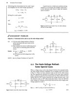
Calculate
the rms
value
of the
periodic triangular
current shown

in Fig.
9.3. Express your answer
in
terms
of
the peak current
I
p
.
-772\
-
Figure
9.3 A
Periodic triangular current.
Solution
From Eq. 9.5, the rms value
of i is
^rms
\l
-T-
Interpreting
the
integral under
the
radical sign
as
the area under
the
squared function
for an

interval
of
one
period
is
helpful
in
finding
the rms
value.
The squared function with
the
area between
0 and
T shaded
is
shown
in
Fig.
9.4,
which also indicates
that
for
this particular function,
the
area under
the
9.2
The
Sinusoidal Response

311
squared current
for an
interval
of one
period
is
equal
to
four times
the
area under
the
squared cur-
rent
for the
interval
0 to TfA
seconds; that
is,
t«+T
/.7/4
i
2
dt = 4 / i
2
dt.
etc.
-7/2-7/4
0

Figure
9.4 • r
versus
t.
7/4 7/2 37/4 7
The analytical expression
for /' in the
interval
0 to
774is
47
i
= -jrt, 0 < / < 774.
The area under
the
squared function
for one
period
is
/
i
2
dt = 4 /
Tlj
r
2
3
The mean,
or
average, value

of the
function
is
simply
the
area
for one
period divided
by the
period. Thus
1
^ - i,2
—
in'
7
3 3
p
'
The
rms
value
of the
current
is the
square root
of
this mean value. Hence
rms
V3'
NOTE: Assess your understanding of this material

by
trying Chapter Problems 9.1, 9.4,
9.8.
9.2 The Sinusoidal Response
Before focusing
on the
steady-state response
to
sinusoidal sources, let's
consider
the
problem
in
broader terms, that
is, in
terms
of the
total
response. Such
an
overview will help
you
keep
the
steady-state solution
in
perspective.
The
circuit shown
in Fig. 9.5

describes
the
general nature
of
the problem. There,
v
s
is a
sinusoidal voltage,
or
v
s
=
V
m
cos
i^t + </>)•
(9.7)
For convenience,
we
assume
the
initial current
in the
circuit
to be
zero
and
measure time from
the

moment
the
switch
is
closed.
The
task
is to
derive
the expression
for /(0
when
t > 0. It is
similar
to
finding
the
step response
of
an RL
circuit,
as in
Chapter
7. The
only difference
is
that
the
voltage
source

is now a
time-varying sinusoidal voltage rather than
a
constant,
or
dc,
voltage. Direct application
of
Kirchhoffs voltage
law to the
circuit
shown
in
Fig.
9.5
leads
to the
ordinary differential equation
Figure
9.5 •
An RL
circuit excited by
a
sinusoidal
voltage source.
L—
+ Ri =
V
m
cos

{a)t
+ 4>\
(9.8)
the formal solution
of
which
is
discussed
in an
introductory course
in dif-
ferential equations.
We ask
those
of you who
have
not yet
studied differ-
ential equations
to
accept that
the
solution
for / is
-v.,
VR
2
+
<o
2

L
2
cos
(0
-6)e~W
L)t
+
V„
VR
2
+
<o
2
L
2
cos
(cot
+
4>
- 0),
(9.9)
where 0 is defined as the angle whose tangent is coL/R. Thus we can easily
determine 0 for a circuit driven by a sinusoidal source of known frequency.
We can check the validity of Eq. 9.9 by determining that it satisfies
Eq. 9.8 for all values of t > 0; this exercise is left for your exploration in
Problem 9.10.
The first term on the right-hand side of Eq. 9.9 is referred to as the
transient component of the current because it becomes infinitesimal as
time elapses. The second term on the right-hand side is known as the
steady-state component of the solution. It exists as long as the switch

remains closed and the source continues to supply the sinusoidal voltage.
In this chapter, we develop a technique for calculating the steady-state
response directly, thus avoiding the problem of solving the differential
equation. However, in using this technique we forfeit obtaining either the
transient component or the total response, which is the sum of the tran-
sient and steady-state components.
We now focus on the steady-state portion of Eq. 9.9. It is important to
remember the following characteristics of the steady-state solution:
1.
The steady-state solution is a sinusoidal function.
2.
The frequency of the response signal is identical to the frequency of
the source signal. This condition is always true in a linear circuit
when the circuit parameters, R, L, and C, are constant. (If frequen-
cies in the response signals are not present in the source signals,
there is a nonlinear element in the circuit.)
3.
The maximum amplitude of the steady-state response, in general,
differs from the maximum amplitude of the source. For the circuit
being discussed, the maximum amplitude of the response signal is
VJ\/R
2
+ arL
2
, and the maximum amplitude of the signal source
is V
m
.
4.
The phase angle of the response signal, in general, differs from the

phase angle of the source. For the circuit being discussed, the phase
angle of the current is
4>
- 0 and that of the voltage source is
<f>.
These characteristics are worth remembering because they help you
understand the motivation for the phasor method, which we introduce in
Section 9.3. In particular, note that once the decision has been made to
find only the steady-state response, the task is reduced to finding the max-
imum amplitude and phase angle of the response signal. The waveform
and frequency of the response are already known.
NOTE: Assess your understanding of this material by trying Chapter
Problem 9.9.
9.3 The Phasor
The phasor is a complex number that carries the amplitude and phase
angle information of a sinusoidal function.
1
The phasor concept is rooted
in Euler's identity, which relates the exponential function to the trigono-
metric function:
e
±jd
= cos6» ± /sin0. (9.10)
Equation 9.10 is important here because it gives us another way of express-
ing the cosine and sine functions. We can think of the cosine function as the
If you feel a bit uneasy about complex numbers, peruse Appendix B.
9.3 The Phasor 313
real part of the exponential function and the sine function as the imaginary
part of the exponential function; that is,
cosfl =

Sfc{tf**},
(9.11)
and
sin0 =
3{<?'
0
},
(9.12)
where 5ft means "the real part of
1
and S means "the imaginary part of."
Because we have already chosen to use the cosine function in analyz-
ing the sinusoidal steady state (see Section 9.1), we can apply Eq. 9.11
directly. In particular, we write the sinusoidal voltage function given by
Eq. 9.1 in the form suggested by Eq. 9.11:
v = V
m
cos
(cot
4-
(f>)
= V
m
$t{e**efi}. (9.13)
We can move the coefficient V
m
inside the argument of the real part of the
function without altering the result. We can also reverse the order of the
two exponential functions inside the argument and write Eq. 9.13 as
V

=
U{V
m
e
jtj>
ei
101
}.
(9.14)
In Eq. 9.14, note that the quantity
V
m
e®
is a complex number that carries
the amplitude and phase angle of the given sinusoidal function. This
complex number is by definition the phasor representation, or phasor
transform, of the given sinusoidal function. Thus
V =
V
m
ef*
= V{V
m
cos(cot + ¢)), (9,15) < Phasor transform
where the notation V{V
m
cos
(cot
+
<f>)}

is read "the phasor transform of
V
m
cos
(cot
4- <£)."Thus the phasor transform transfers the sinusoidal func-
tion from the time domain to the complex-number domain, which is also
called the frequency domain, since the response depends, in general, on to.
As in Eq. 9.15, throughout this book we represent a phasor quantity by
using a boldface letter.
Equation 9.15 is the polar form of a phasor, but we also can express a
phasor in rectangular form. Thus we rewrite Eq. 9.15 as
V = V
m
cos $ + jV
m
sin
</>.
(9.16)
Both polar and rectangular forms are useful in circuit applications of the
phasor concept.
One additional comment regarding Eq. 9.15 is in order. The frequent
occurrence of the exponential function e^ has led to an abbreviation that
lends itself to text material. This abbreviation is the angle notation
We use this notation extensively in the material that follows.
Inverse Phasor Transform
So far we have emphasized moving from the sinusoidal function to its pha-
sor transform. However, we may also reverse the process. That is, for a
phasor we may write the expression for the sinusoidal function. Thus for
V = l()0/-26°, the expression for v is 100cos

(a)t
- 26°) because we
have decided to use the cosine function for all sinusoids. Observe that we
cannot deduce the value of
co
from the phasor. The phasor carries only
amplitude and phase information. The step of going from the phasor
transform to the time-domain expression is referred to as finding the
inverse phasor transform and is formalized by the equation
V~
x
{V
m
e^}
= $t{V
m
e
i4
>e>
m
}, (9.17)
where the notation
V~
l
{V
m
e^}
is read as "the inverse phasor transform of
V
m

e'^."
Equation 9.17 indicates that to find the inverse phasor transform, we
multiply the phasor by <?
/W
and then extract the real part of the product.
The phasor transform is useful in circuit analysis because it reduces
the task of finding the maximum amplitude and phase angle of the steady-
state sinusoidal response to the algebra of complex numbers. The follow-
ing observations verify this conclusion:
1.
The transient component vanishes as time elapses, so the steady-
state component of the solution must also satisfy the differential
equation. (See Problem 9.10[b].)
2.
In a linear circuit driven by sinusoidal sources, the steady-state
response also is sinusoidal, and the frequency of the sinusoidal
response is the same as the frequency of the sinusoidal source.
3.
Using the notation introduced in Eq.
9.11,
we can postulate that the
steady-state solution is of the form lR{Ae'
li
e
JM
'}, where A is the
maximum amplitude of the response and /3 is the phase angle of the
response.
4.
When we substitute the postulated steady-state solution into the

differential equation, the exponential term
e
,u>l
cancels out, leaving
the solution for A and ft in the domain of
complex numbers.
We illustrate these observations with the circuit shown in Fig. 9.5 (see
p.
311).
We
know that the steady-state solution for the current i is of the form
WO = K{//fl, (9.18)
where the subscript
u
ss" emphasizes that we are dealing with the steady-
state solution. When we substitute Eq. 9.18 into Eq. 9.8, we generate the
expression
®.{}<oLI
m
e®ei«*}
+ n{RI
m
e
iP
e
J(M
} = ^{V
m
e^
wt

\. (9.19)
In deriving Eq. 9.19 we recognized that both differentiation and multiplica-
tion by a constant can be taken inside the real part of an operation. We also
rewrote the right-hand side of Eq. 9.8, using the notation of Eq.
9.11.
From
the algebra of complex numbers, we know that the sum of the real parts is the
same as the real part of the sum. Therefore we may reduce the left-hand side
of Eq. 9.19 to a single term:
9R{(/wL + K^'V*} =
ftlV^V*"}.
(9.20)
Recall that our decision to use the cosine function in analyzing the
response of a circuit in the sinusoidal steady state results in the use of
the 5ft operator in deriving Eq. 9.20. If instead we had chosen to use the
sine function in our sinusoidal steady-state analysis, we would have
applied Eq. 9.12 directly, in place of Eq. 9.11, and the result would be
Eq.9.21:
Q{(j(ol + R)I
m
e
ifi
e^} =
^{V
m
e
j
^
wt
}.

(9.21)
Note that the complex quantities on either side of Eq. 9.21 are identical to
those on either side of Eq.
9.20.
When both the real and imaginary parts of
two complex quantities are equal, then the complex quantities are them-
selves equal. Therefore, from Eqs. 9.20 and 9.21,
(J(oL + R)I
m
e® = V
m
e
i<!>
or
<-*
- OiZ
(9
-
22
>
Note that
e
Ja>t
has been eliminated from the determination of the ampli-
tude (/,„) and phase angle (/3) of the response. Thus, for this circuit, the
task of finding /,„ and /3 involves the algebraic manipulation of the com-
plex quantities
V
m
e®

and R + jwL. Note that we encountered both polar
and rectangular forms.
An important warning is in order: The phasor transform, along with
the inverse phasor transform, allows you to go back and forth between
the time domain and the frequency domain. Therefore, when you obtain
a solution, you are either in the time domain or the frequency domain.
You cannot be in both domains simultaneously. Any solution that con-
tains a mixture of time domain and phasor domain nomenclature is
nonsensical.
The phasor transform is also useful in circuit analysis because it applies
directly to the sum of sinusoidal functions. Circuit analysis involves sum-
ming currents and voltages, so the importance of this observation is obvi-
ous.
We can formalize this property as follows: If
v = Vi + Vj + ••• + v
n
(9.23)
where all the voltages on the right-hand side are sinusoidal voltages of the
same frequency, then
v
= v,
-+-v
2
+ ••• +
v„.
(9.24)