Electric Circuits, 9th Edition P36 docx

326 Sinusoidal Steady-State Analysis
^ASSESSMENT PROBLEMS
Objective 3—Know how to use circuit analysis techniques to solve a circuit in the frequency domain
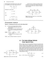
9.7 A 20 fl resistor is connected in parallel with a
5 mH inductor. This parallel combination is
connected in series with a 5 ft resistor and a
25 ^iF capacitor.
a) Calculate the impedance of this inter-
connection if the frequency is 2 krad/s.
b) Repeat (a) for a frequency of 8 krad/s.
c) At what finite frequency does the imped-
ance of the interconnection become purely
resistive?
d) What is the impedance at the frequency
found in (c)?
NOTE: Also try Chapter Problems 9.28, 9.29, and 9.32.
Answer: (a) 9 - /12 fl;
(b) 21 + /3 O;
(c) 4 krad/s;
(d) 15 ft,
9.8 The interconnection described in Assessment
Problem 9.7 is connected across the terminals
of a voltage source that is generating
v = 150 cos 4000f V. What is the maximum
amplitude of the current in the 5 mH inductor?
Answer: 7.07 A.
Figure 9.20 •
The
delta-to-wye transformation.
Delta-to-Wye Transformations
The A-to-Y transformation that we discussed in Section 3.7 with regard

to resistive circuits also applies to impedances. Figure 9.20 defines the
A-connected impedances along with the Y-equivalent circuit. The
Y impedances as functions of the A impedances are
(9.51)
Z
3
z, =
z
d
z.
ZbZ
c
+ z
b
+ z;
Z
C
Z,
A
+ z
b
+
z»z
b
z/
z, + z
h
+ z
c
(9.52)

(9.53)
The A-to-Y transformation also may be reversed; that is, we can start
with the Y structure and replace it with an equivalent A structure. The A
impedances as functions of the Y impedances are
Z, =
Z\Z
2
ZiZ
2
Z)Z
2
+ Z
2
Zi
Z\
+
Z
2
Z
3
z
2
+
z
2
z
3
+ Z
3
Zi

+
z
3
z
x
+
Zj,Z
x
z,
(9.54)
(9.55)
(9.56)
The process used to derive Eqs. 9.51-9.53 or Eqs. 9.54-9.56 is the same
as that used to derive the corresponding equations for pure resistive cir-
cuits.
In fact, comparing Eqs. 3.44-3.46 with Eqs. 9.51-9.53, and
Eqs.
3.47-3.49 with Eqs. 9.54-9.56, reveals that the symbol Z has replaced
9.6 Series, Parallel, and Delta-to-Wye Simplifications 327
the symbol R. You may want to review Problem 3.62 concerning the deri-
vation of the A-to-Y transformation.
Example 9.8 illustrates the usefulness of the A-to-Y transformation in
phasor circuit analysis.
Example 9.8 Using a Delta-to-Wye Transform in the Frequency Domain
Use a A-to-Y impedance transformation to find I
()
,
Ii,
I
2

,13,14,15, V|, and V
2
in the circuit in Fig. 9.21.
C_)
12(M£
Figure 9.21 A The circuit for Example 9.8.
Solution
First note that the circuit is not amenable to series
or parallel simplification as it now
stands.
A A-to-Y
impedance transformation allows us to solve for all
the branch currents without resorting to either the
node-voltage or the mesh-current method. If we
replace either the upper delta (abc) or the lower
delta (bed) with its Y equivalent, we can further
simplify the resulting circuit by series-parallel com-
binations. In deciding which delta to replace, the
sum of the impedances around each delta is worth
checking because this quantity forms the denomi-
nator for the equivalent Y impedances. The sum
around the lower delta is 30 + /40, so we choose to
eliminate it from the circuit. The Y impedance con-
necting to terminal b is
(21) + /60)(10)
Zl =
30 + /40
= 12 +
>
4a

'
the Y impedance connecting to terminal c is
10(-/20)
and the Y impedance connecting to terminal d is
(20 + ;60)(-y20)
Inserting the Y-equivalent impedances into the cir-
cuit, we get the circuit shown in Fig 9.22, which we
can now simplify by series-parallel reductions. The
impedence of the abn branch is
Z
ahn
= 12 + ./4 - /4 = 12 ft,
and the impedance of the acn branch is
Z
acn
= 63.2 + /2.4 - /2.4 - 3.2 = 60 ft.
4ft
-/2.4 ft
Figure 9.22 • The circuit shown in Fig. 9.21, with the lower
delta replaced by its equivalent wye.
Note that the abn branch is in parallel with the acn
branch.
Therefore we may replace these two branches
with a single branch having an impedance of
•^an
(60)(12)
72
10 ft.
Combining this 10 ft resistor with the impedance
between n and d reduces the circuit shown in Fig. 9.22

to the one shown in
Fig.
9.23.
From the latter circuit.
120/0°
h = 7Z ~. =4/53.13°
1
18 - /24
l
2.4 + /3.2 A.
Z
3
=
30 + /40
= 8 - /24 ft.
Once we know I
()
, we can work back through the
equivalent circuits to find the branch currents in
the original circuit. We begin by noting that I
0
is
the current in the branch nd of Fig. 9.22. Therefore
V
nd
= (8 - /24)1« = 96 - /32 V.
328 Sinusoidal Steady-State Analysis
We may now calculate the voltage V
an
because

*
T
an
'
T
nd
and both V and V
nd
are known. Thus
V
an
= 120 - 96 + /32 = 24 + /32 V.
We now compute the branch currents I
abn
and I
acn
:
24 + /32 .8
A
Iabn = J^ = 2 + J ~ A,
24 + /32 _ _4_ _8_
60 " ~ 10
+ ;
15
A
"
In terms of the branch currents defined in Fig. 9.21,
Ii = Iabn = 2 + /3
A
'

i_ •_§_
10
+7
15
h = Iacn = T7T + 777
A
«
We check the calculations of Ii and I? by noting that
I, + I
2
= 2.4 + /3.2 = I
0
.
•V
a
120/Q!/
+
V
i8n
-/2412
Figure 9.23 • A simplified version of the circuit shown in
Fig.
9.22.
To find the branch currents I
3
, I
4
, and I
5
, we must

first calculate the voltages V! and V
2
. Refering to
Fig. 9.21, we note that
328
V
t
= 120/CT -
(-/4)1,
= — + /8 V,
V
2
= 120/0° - (63.2 + /2.4)I
2
= 96 - j~ V.
We now calculate the branch currents
I
3
,1
4
,
and I
5
;
V
L
- V
2
4 . 12.8
13 = -^- = 3 +i— A,

l4 =
2^T7rS
=
3"
7l
-
6A
'
^-g**"-
We check the calculations by noting that
I
4
+ Is = 3 + jg - /1-6 + /4.8 = 2.4 + /3.2 = I
0
,
4 2
12.8
M
, „ .8
w
I3 + I
4
= 3 + 3 + ;— - ;1.6 = 2 + 7- = l
h
4 4 12.8 8 26
•/ASSESSMENT PROBLEM
Objective 3—Know how to use circuit analysis techniques to solve a circuit in the frequency domain
9.9 Use a
A
-to-Y transformation to find the

current I in the circuit shown. 1 ^
I
Answer: I = 4 /28.07° A.
136zD!/+^
1411
/40 fl ^ -/15 H
ion
NOTE: Also try Chapter Problem 9.37.
9.7 Source Transformations and Thevenin-Norton Equivalent Circuits 329
9 J Source Transformations and
Thevenin-Norton Equivalent Circuits
The source transformations introduced in Section 4.9 and the Thevenin-
Norton equivalent circuits discussed in Section 4.10 are analytical tech-
niques that also can be applied to frequency-domain circuits. We prove
the validity of these techniques by following the same process used in
Sections 4.9 and 4.10, except that we substitute impedance (Z) for resist-
ance (/?). Figure 9.24 shows a source-transformation equivalent circuit
with the nomenclature of the frequency domain.
Figure 9.25 illustrates the frequency-domain version of a Thevenin
equivalent circuit. Figure 9.26 shows the frequency-domain equivalent of
a Norton equivalent circuit. The techniques for finding the Thevenin
equivalent voltage and impedance are identical to those used for resistive
circuits, except that the frequency-domain equivalent circuit involves the
manipulation of complex quantities. The same holds for finding the
Norton equivalent current and impedance.
Example 9.9 demonstrates the application of the source-transformation
equivalent circuit to frequency-domain analysis. Example 9.10 illustrates
the details of finding a Thevenin equivalent circuit in the frequency domain.
Z
s

v,/z.
Figure 9.24 A A source transformation in the
frequency domain.
Frequency-domain
linear circuit;
may contain
both independent
and dependent
sources. •"
Figure 9.25 • The frequency-domain version of a
Thevenin equivalent circuit.
Frequency-domain
linear circuit;
may contain
both independent
and dependent ,
sources. *
b
Figure 9.26 • The frequency-domain version of
a
Norton
equivalent circuit.
Example 9.9
Performing Source Transformations in the Frequency Domain
Use the concept of source transformation to find the
phasor voltage V
0
in the circuit shown in Fig. 9.27.
in
y'3

0 0.2 a
;'°-
6a
I "WV rv-w>—^_/yy\,
ry\~r\
^
/^ + \40ZQ!
Figure 9.27 A The circuit for Example 9.9.
Solution
We can replace the series combination of the
voltage source (40/0°) and the impedance of
1 +/3Q with the parallel combination of a
current source and the 1 + /3 ft impedance. The
source current is
I =
TTp
=
To
(1
-
;3)
/12 A.
Thus we can modify the circuit shown in Fig. 9.27 to
the one shown in Fig. 9.28. Note that the polarity
reference of the 40 V source determines the refer-
ence direction for I.
Next, we combine the two parallel branches
into a single impedance,
Z =
(1 + /3)(9 - /3)

10
= 1.8 + /2.4 a,
330 Sinusoidal Steady-State Analysis
which is in parallel with the current source of
4 - y*12 A. Another source transformation con-
verts this parallel combination to a series combina-
tion consisting of a voltage source in series with the
impedance of 1.8 + /2.4 ft. The voltage of the volt-
age source is
V = (4 - /12)(1.8 + /2.4) = 36 - /12 V.
Using this source transformation, we redraw the
circuit as Fig. 9.29. Note the polarity of the voltage
source. We added the current Io to the circuit to
expedite the solution for
VQ.
0.2 0, /0.6 H
>VvV '^YYV
Figure 9.28 • The first step in reducing the circuit shown
in Fig. 9.27.
1.8
n
/2.4
n
o.2
o
/o.6
n
l /\/W orw-\ /y^
OTTTL
c

Figure 9.29 • The second step in reducing the circuit shown
in Fig. 9.27.
Also note that we have reduced the circuit to a
simple series circuit. We calculate the current Io by
dividing the voltage of the source by the total series
impedance:
=
36 - /12
=
12(3 - /1)
0
12 - /16 ~ 4(3 - /4)
39 + /27
25
1.56 +/1.08 A.
We now obtain the value of V
0
by multiplying I
0
by
the impedance 10 - /19:
V
fl
= (1.56 + /1.08)(10 - /19) = 36.12 - /18.84 V.
Example 9.10
Finding a Thevenin Equivalent in the Frequency Domain
Find the Thevenin equivalent circuit with respect to
terminals a,b for the circuit shown in Fig. 9.30.
12
H

-/40 a
no a
120ffi(^
v
J
6Qn
^
10Vj
Figure 9.30 • The circuit for Example 9.10.
Solution
We first determine the Thevenin equivalent voltage.
This voltage is the open-circuit voltage appearing at
terminals a,b. We choose the reference for the
Thevenin voltage as positive at terminal a. We can
make two source transformations relative to the
120
V,
12
CI,
and 60
CI
circuit elements to simplify this
portion of the
circuit.
At the same time, these transfor-
mations must preserve the identity of the controlling
voltage Vj because of the dependent voltage source.
We determine the two source transformations by
first replacing the series combination of the 120 V
source and 12

CI
resistor with a 10 A current source
in parallel with 12
CI.
Next, we replace the parallel
combination of the 12 and 60 ft resistors with a single
10 ft resistor. Finally, we replace the 10 A source in
parallel with 10 ft with a 100 V source in series with
10 ft. Figure 9.31 shows the resulting circuit.
We added the current I to Fig. 9.31 to aid fur-
ther discussion. Note that once we know the current
9.7 Source Transformations and Thevenin-Norton Equivalent Circuits 331
I, we can compute the Thevenin voltage. We find I
by summing the voltages around the closed path in
the circuit shown in Fig. 9.31. Hence
100 = 101 - /401 + 1201 + 10V
t
= (130 - /40)1 + 10V
V
.
-/40 ft
100/0!'
V
I
120 ft
'WV-
10
V
v
-•a

+
v-
ni
Figure 9.32 A A circuit for calculating the Thevenin equivalent
impedance.
Figure 9.31 •
A
simplified version of
the
circuit shown
in
Fig.
9.30.
We relate the controlling voltage V
v
to the current I
by noting from Fig. 9.31 that
'Hi en,
V
v
= 100 - 101.
= 18/-126.87° A.
30 - /40
we now calculate V
x
:
V
v
= 100 - 180/-126.87° = 208 + /144 V.
Finally, we note from Fig. 9.31 that

V-rh = 10¼ + 1201
= 2080 + /1440 + 120(18)/-126.87°
= 784 - /288 = 835.22/-20.17° V.
To obtain the Thevenin impedance, we may
use any of the techniques previously used to find
the Thevenin resistance. We illustrate the test-
source method in this example. Recall that in
using this method, we deactivate all independent
sources from the circuit and then apply either a
test voltage source or a test current source to the
terminals of interest. The ratio of the voltage to
the current at the source is the Thevenin imped-
ance.
Figure 9.32 shows the result of applying this
technique to the circuit shown in Fig. 9.30. Note
that we chose a test voltage source \
T
. Also note
that we deactivated the independent voltage
source with an appropriate short-circuit and pre-
served the identity of V
v
.
The branch currents I
a
and I
b
have been added to
the circuit to simplify the calculation of I
T

. By
straightforward applications of Kirchhoff s circuit
laws,
you should be able to verify the following
relationships:
Ih =
10 - /40
v
r
- iov
A
120
_ -V
7
(9 + /4)
' 120(1 - /4) *
IT = la + lb
^ V, = 10I
a
,
V
r
f 9 + /4
10 - /40
V
12
VH3-/4)
' 12(10-/40)
1
Z-n,

= T
1
= 91.2
-/38.411.
If
Figure 9.33 depicts the Thevenin equivalent circuit.
784-/288/
+
V
91.2 ft
/yyV—
-/38.4X2
+
Figure 9.33 • The Thevenin equivalent for the circuit shown
in
Fig.
9.30.
332 Sinusoidal Steady-State Analysis
/ASSESS MEN
Objective 3—Know how to use circuit analysis techniques to solve a circuit in the frequency domain
9.10 Find the steady-state expression for v
0
{t) in
the circuit shown by using the technique of
source transformations. The sinusoidal voltage
sources are
v
x
= 240 cos (4000/ + 53.13°) V,
th = 96 sin 4000/ V.

20
H
Answer: 48 cos (4000/ + 36.87°) V
NOTE: Also try Chapter Problems 9.45, 9.46, and 9.49.
9.11 Find the Thevenin equivalent with respect to
terminals a,b in the circuit shown.
Answer: V
Th
= V
ab
= 10/45^ V;
Z
Th
= 5 - /5 H.
9.8 The Node-Voltage Method
In Sections 4.2-4.4, we introduced the basic concepts of the node-voltage
method of circuit analysis. The same concepts apply when we use the
node-voltage method to analyze frequency-domain circuits. Example 9.11
illustrates the solution of such a circuit by the node-voltage technique.
Assessment Problem 9.12 and many of the Chapter Problems give you an
opportunity to use the node-voltage method to solve for steady-state sinu-
soidal responses.
Example 9.11
Using the Node-Voltage Method in the Frequency Domain
Use the node-voltage method to find the branch
currents I
a
, I
b
, and I

c
in the circuit shown in
Fig.
9.34.
Figure 9.34 •
The
circuit for Example 9.11.
Solution
We can describe the circuit in terms of two node volt-
ages because it contains three essential nodes. Four
branches terminate at the essential node that stretches
across the bottom of
Fig.
9.34,
so we use it as the refer-
ence node. The remaining two essential nodes are
labeled
1
and
2,
and the appropriate node voltages are
designated V] and V
2
. Figure 9.35 reflects the choice
of reference node and the terminal labels.
10.6/0!
A
1 lft /2 ft 2
5
a

f WV rwy~\—« ,yvV-
Mj 100
Figure 9.35 A
The
circuit shown in Fig. 9.34, with the node
voltages defined.
Summing the currents away from node 1 yields
Vi Vi - V
7
-10.6 + 777 + -r ~ = °-
10 1 + j2
Multiplying by 1 + /2 and collecting the coeffi-
cients of V] and V
2
generates the expression
V^l.l + /0.2) - V
2
= 10.6 + /21.2.
9.9 The Mesh-Current Method 333
Summing the currents away from node 2 gives
V2-V1 , V
2
, V
2
~ 201
+ 1 = U.
1 + /2 -/5 5
The controlling current I, is
I,
1 + /2

Substituting this expression for l
x
into the node 2
equation, multiplying by 1 + /2, and collecting
coefficients of V, and V
2
produces the equation
-5V
t
+ (4.8 + /0.6) V
2
= 0.
The solutions for V^ and V
2
are
V! = 68.40 -/16.80 V,
V
2
= 68 - /26 V.
Hence the branch currents are
I
a
= ^ = 6.84-/1.68 A,
Vi - V
2
1 +/2
= 3.76 + /1.68 A,
V
2
- 20I

X
I
b
= -*— = -1.44 - /11.92 A,
V,
I
c
= -^+ = 5.2 + /13.6 A.
-;5
To check our work, we note that
I
a
+ I, = 6.84 - /1.68 + 3.76 + /1.68
= 10.6 A,
I
v
= I
b
+ I
c
= -1.44 - /11.92 + 5.2 + /13.6
= 3.76 + /1.68 A.
^ASSESSMENT PROBLEM
Objective 3—Know how to use circuit analysis techniques to solve a circuit in the frequency domain
9.12 Use the node-voltage method to find the steady-
state expression for v(t) in the circuit shown. The
sinusoidal sources are i
s
= 10 cos
cot

A and
v
s
= 100 sin
cot
V, where to - 50 krad/s.
Answer: v(t) = 31.62 cos (50,000r - 71.57°) V.
NOTE: Also try Chapter Problems 9.55 and 9.59.
20
a
9.9 The Mesh-Current Method
We can also use the mesh-current method to analyze frequency-domain cir-
cuits.
The procedures used in frequency-domain applications are the same
as those used in analyzing resistive circuits. In Sections 4.5-4.7, we intro-
duced the basic techniques of the mesh-current method; we demonstrate
the extension of this method to frequency-domain circuits in Example 9.12.
Example 9.12
Using the Mesh-Current Method in the Frequency Domain
Use the mesh-current method to find the voltages
Vj,
V
2
,and V
3
in the circuit shown in Fig. 9.36 on the
next page.
Solution
The circuit has two meshes and a dependent volt-
age source, so we must write two mesh-current

equations and a constraint equation. The reference
direction for the mesh currents I] and I
2
is clock-
wise,
as shown in Fig. 9.37. Once we know ^ and I
2
,
we can easily find the unknown voltages. Summing
the voltages around mesh
1
gives
150 = (1 +/2)^ + (12-/16)(1, -I
2
),
or
150 = (13 - /14)¾ - (12 - /16)I
2
.
Summing the voltages around mesh 2 generates the
equation
0 = (12 - /16)(¾ - 10 + (1+ /3)¾ + 391,.
Figure 9.37 reveals that the controlling current I, is
the difference between I, and I
2
; that is, the con-
straint is
Ir = It - h
334 Sinusoidal Steady-State Analysis
+ V, - + V,

I VvV L_rY-w-\ m /y^ L_TY>nr\_
ui yzn+T m
/3
a
120¾
O'T
v
=
-;'16ft:
39
I
A
Figure 9.36 •
The
circuit for Example 9.12.
1 fl /2
A 1
(1 /3
£1
i <wv o"v>-> • »yy^ orw>_
Solving for I] and I
2
yields
I, = -26- /52 A,
I
2
= -24 - /58 A,
I
v
= -2 + /6 A.

The three voltages are
Vj = (1 + /2)1
1
= 78 -/104 V,
V
2
= (12 -
/16)1,
= 72 + /104 V,
V
3
= (1 + /3)I
2
= 150 - /130 V.
Also
391
v
= -78 + /234 V.
Figure 9.37 • Mesh currents used to solve the circuit shown
in
Fig.
9.36.
Substituting this constraint into the mesh 2 equa-
tion and simplifying the resulting expression gives
0 = (27 + /16)¾ - (26 + /13)¾.
We check these calculations by summing the volt-
ages around closed paths:
-150 + Vj + V
2
= -150 + 78 - /104 + 72

+ /104 = 0,
-V
2
+ V
3
+ 39¾ = -72 - /104 + 150 - /130
- 78 + /234 = 0,
-150 + V! + V
3
+
39¾.
= -150 + 78 - /104 + 150
- /130 - 78 + /234 = 0.
^ASSESSMENT PROBLEM
Objective 3—Know how to use circuit analysis techniques to solve a circuit in the frequency domain
9.13 Use the mesh-current method to find the pha-
sor current I in the circuit shown.
Answer: I = 29 + /2 = 29.07/3.95° A.
NOTE: Also try Chapter Problems 9.60 and 9.64.
/^+^33.8/0°
9.10 The Transformer
A transformer is a device that is based on magnetic coupling. Transformers
are used in both communication and power circuits. In communication cir-
cuits,
the transformer is used to match impedances and eliminate dc signals
from portions of the system. In power circuits, transformers are used to estab-
lish ac voltage levels that facilitate the transmission, distribution, and con-
sumption of electrical power. A knowledge of the sinusoidal steady-state
9.10
The

Transformer 335
behavior of the transformer
is
required in the analysis of both communication
and power systems. In this section, we will discuss the sinusoidal steady-state
behavior of the linear transformer, which is found primarily in communica-
tion circuits. In Section
9.11,
we will deal with the ideal transformer, which is
used to model the ferromagnetic transformer found in power systems.
Before starting we make a useful observation. When analyzing circuits
containing mutual inductance use the meshor loop-current method for writ-
ing circuit equations. The node-voltage method is cumbersome to use when
mutual inductance in involved. This is because the currents in the various
coils cannot be written by inspection as functions of the node voltages.
The Analysis of a Linear Transformer Circuit
A simple transformer is formed when two coils are wound on a single core
to ensure magnetic coupling. Figure 9.38 shows the frequency-domain cir-
cuit model of a system that uses a transformer to connect a load to a
source. In discussing this circuit, we refer to the transformer winding con-
nected to the source as the primary winding and the winding connected to
the load as the secondary winding. Based on this terminology, the trans-
former circuit parameters are
jR] = the resistance of the primary winding,
R
2
= the resistance of the secondary winding,
Lj = the self-inductance of the primary winding,
L
2

- the self-inductance of the secondary winding.
M = the mutual inductance.
The internal voltage of the sinusoidal source is V
v
, and the internal
impedance of the source is Z
s
. The impedance Z
L
represents the load con-
nected to the secondary winding of the transformer. The phasor currents
Ij and I
2
represent the primary and secondary currents of the transformer,
respectively.
Analysis of the circuit in Fig. 9.38 consists of finding I, and I
2
as func-
tions of the circuit parameters V
v
, Z
s
, R
h
L
t
, L
2
, R
2

, M, Z
L
, and
OJ.
We are
also interested in finding the impedance seen looking into the transformer
from the terminals a,b.To find l\ and I
2
, we first write the two mesh-cur-
rent equations that describe the circuit:
Source
Transformer Load
Figure 9.38 A The frequency domain circuit model for a
transformer used to connect a load to a source.
V
v
= (Z
v
+ Ri + jo)L
l
)l
l
- ja>Ml
2
,
(9.57)
0 = -;©Afl| + (R
2
+ joiL
2

4- Z
L
)I
2
. (9.58)
To facilitate the algebraic manipulation of Eqs. 9.57 and 9.58, we let
Z,,
= Z, + R
x
+ jtoL
u
(9.59)
Z
22
= R
2
+ jcoL
2
+
ZJL,
(9.60)
where Z
(1
is the total self-impedance of the mesh containing the primary
winding of the transformer, and Z
22
is the total self-impedance of the
mesh containing the secondary winding. Based on the notation introduced
in Eqs. 9.59 and 9.60, the solutions for Ij and I
2

from Eqs. 9.57 and 9.58 are
I. =
Z
]]
Z
22
4-
o)~M
V
~>
* 17
x
'
(9.61)
JOjM
Z
U
Z
22
+ w'M
io)M
-V = - 1,
(9.62)
'22