Electric Circuits, 9th Edition P49 docx

Observe that the right-hand side of Eq. 12.96 may be written as
lim / -j-e"dt + / -^e~
st
dt .
*-°°\
Mr dt J
it
dt J
As s
—*
co, (df/dt)e~
st
—>
0; hence the second integral vanishes in the limit.
The first integral reduces to /(0
+
) -
/(0~),
which is independent of s. Thus
the right-hand side of Eq. 12.96 becomes
lim / %e-
u
dt = /(0
+
) -
/(0-).
(12.97)
Because /(0
-
) is independent of s, the left-hand side of Eq. 12.96 may
be written

lim[5F(j) - /(0^)1 = Iim[sF(s)] -
/(0
-
).
(12.98)
From Eqs. 12.97 and 12.98,
limsF(s) =/(0
+
) = lim/(/),
which completes the proof of the initial-value theorem.
The proof of the final-value theorem also starts with Eq. 12.95. Here
we take the limit as s
—>
0:
lim[^) - /(0-)] = Km(y_
Yt
e
~
St(lt
)-
(12
-
99)
The integration is with respect to t and the limit operation is with respect
to s, so the right-hand side of Eq. 12.99 reduces to
limf / -j-e'^dt) = / -f dt. (12.100)
Because the upper limit on the integral is infinite, this integral may also be
written as a limit process:
df f'df
dt = lim / -r-dy,

(12.101)
0-
dt ,^oc
J
Q
-dy
•
where we use y as the symbol of integration to avoid confusion with the
upper limit on the integral. Carrying out the integration process yields
lim [/(0 - /(0-)] = lim
[/(f)]
-
/(0-).
(12.102)
Substituting Eq. 12.102 into Eq. 12.99 gives
lim[^(5')] - /(0-) = lim [/(0] -
/(0-).
(12.103)
s—*\)
t—*cc
Because /(0
-
)
cancels,
Eq. 12.103 reduces to the final-value theorem, namely,
limA'F(s) = lim/(0-
The final-value theorem is useful only if /(°°) exists.This condition is true
only if all the poles of F(s), except for a simple pole at the origin, lie in the
left half of the s plane.
12.9 Initial- and Final-Value Theorems

The Application of Initial- and Final-Value Theorems
To illustrate the application of the initial- and final-value theorems, we
apply them to a function we used to illustrate partial fraction expan-
sions.
Consider the transform pair given by Eq. 12.60. The initial-value
theorem gives
100s
2
[l + (3/s)]
Jim sF(s) = lim -: =— = 0,
s
^oo
v
'
s-*™
s
\\
+ (6/s))[l + (6/.9) + (25/5
2
)]
lim /(0 = [-12 + 20cos(-53.13°)](l) = -12 + 12 = 0.
The final-value theorem gives
lQOsjs + 3)
•o
i—o (
s
+
6)(5:
2
+ 6s + 25)

lim sF(s) = lim — ^
w 2
7777T
=
^»
lim f{t) = lim[-12e~
6r
+ 20e
_3
'cos(4f - 53.13°)]w(f) = 0.
t—>00 /—»00
In applying the theorems to Eq.
12.60,
we already had the time-domain
expression and were merely testing our understanding. But the real value of
the initial- and final-value theorems lies in being able to test the .s-domain
expressions before working out the inverse transform. For example, con-
sider the expression for V(s) given by Eq.
12.40.
Although we cannot calcu-
late v(t) until the circuit parameters are specified, we can check to see if
V(s) predicts the correct values of v(0
+
) and ?;(oo). We know from the
statement of the problem that generated V(s) that v(0
+
) is zero. We also
know that v(oo) must be zero because the ideal inductor is a perfect short
circuit across the dc current source. Finally, we know that the poles of V(s)
must lie in the left half of the s plane because R, L, and C are positive con-

stants.
Hence the poles of sV(s) also lie in the left half of the s plane.
Applying the initial-value theorem yields
lim sV(s) = lim
s(I
dc
/Q
s-+°os
2
[\
+ \/(RCs) + \/{LCs
2
)]
Applying the final-value theorem gives
s(hc/C)
lim sV(s) = lim ^: = 0.
5-o ,-o
5
2
+ (s/RC) + (1/LC)
The derived expression for V(s) correctly predicts the initial and final val-
ues of v(t).
/"ASSESSMENT PROBLEM
Objective 3—Understand and know how to use the initial value theorem and the final value theorem
12.10 Use the initial- and final-value theorems to find Answer: 7,0;
4,1;
and 0,0.
the initial and final values of f(t) in Assessment
Problems 12.4,12.6, and 12.7.
NOTE: Also try Chapter Problem 12.50.

458 Introduction
to
the Laplace Transform
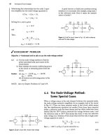
Practical Perspective
Transient Effects
The circuit introduced
in the
Practical Perspective
at the
beginning
of the
chapter
is
repeated
in Fig. 12.18
with
the
switch closed
and the
chosen
sinusoidal source.
10mH
m
»
F
cosl2(hrfV( £15 a
Figure 12.18
A
A
series

RLC
circuit with
a
60 Hz
sinusoidal source.
We
use the
Laplace methods
to
determine
the
complete response
of the
inductor current,
4(0-
TO
begin,
use
KVL
to
sum
the
voltages drops around
the circuit,
in the
clockwise direction:
15i
L
(t) + 0.01-¾^ + -r /
i

L
(x)dx
= cosUOTrt (12.104)
at 100 X 10 \/o
Now we take the Laplace transform
of
Eq.
12.104, using Tables 12.1 and
12.2:
15/
L
(5) + 0.01s/
L
(5) + 10
4
-^ = -= / -r (12.105)
Next, rearrange
the
terms
in
Eq. 12.105
to get
an expression
for
I
L
(s):
100s
2
Ids) = 7- -rrz r-T (12.106)

[5
2
+ 15005 + 10
6
][5
2
+
(120TT
2
)]
Note that
the
expression
for 4(^) has two
complex conjugate pairs
of
poles,
so the
partial fraction expansion
of I
L
(s)
will have four terms:
L(
^
=
(5 + 750 - /661.44)
+
(5 + 750 + /661.44)
+

(5 -
/120TT)
+
(5 +
;120TT)
(12.107)
Determine
the
values
of K\
and
K
2
*
IOO5
2
K
Y
=
K
7
=
5 + 7505 + /661.44]
[5
2
+
(120TT)
2
]
IOO5

2
= 0.07357Z-97.89
0
5=-750+/661.44
[5
2
+ 15005 + 10
6
][5 + /120V]
(12.108)
= 0.018345
Z
56.61°
s=/120w
Finally,
we can
use Table
12.3 to
calculate
the
inverse Laplace transform
of
Eq.
12.107
to
give
4(/):
4(0 = 147.14*T
750
' cos(661.44f - 97.89°) + 36.69

COS(120TT?
+ 56.61°) mA (12.109)
The first term
of
Eq. 12.109
is the
transient response, which will decay
to
essentially zero
in
about
7
ms. The second term
of
Eq. 12.109
is the
steady-
state response, which has
the
same frequency as
the 60
Hz sinusoidal source
and will persist
so
long as this source
is
connected
in the
circuit. Note that
the amplitude

of
the steady-state response
is
36.69
mA,
which
is
less than
the
40 mA
current rating
of
the inductor.
But the
transient response
has an
Summary 459
initial amplitude of 147.14 mA, far greater than the 40 mA current rating.
Calculate the value of the inductor current at t — 0:
i
£
(0) = 147.14(l)cos(-97.89°) + 36.69 cos(56.61°) = -6.21/xA
Clearly, the transient part of the response does not cause the inductor current to
exceed its rating initially. But we need a plot of the complete response to deter-
mine whether or not the current rating is ever
exceeded,
as shown in Fig. 12.19.
The plot suggests we check the value of the inductor current at 1 ms:
;
L

(0.001) = 147.14e
_0J5
cos(-59.82°) + 36.69 cos(78.21°) = 42.6 mA
Thus,
the current rating is exceeded in the inductor, at least momentarily. If
we determine that we never want to exceed the current rating, we should
reduce the magnitude of the sinusoidal source. This example illustrates the
importance of considering the complete response of a circuit to a sinusoidal
input, even if we are satisfied with the steady-state response.
^(mA)
50
1
Figure 12.19 A Plot of
the
inductor current for the circuit in Fig. 12.18.
NOTE:
Access
your understanding of the Practical Perspective by trying Chapter
Problems
12.55 and 12.56.
Summary
K is the strength of the impulse; if K = 1, K8(t) is the
unit impulse function. (See page 433.)
A functional transform is the Laplace transform of a
specific function. Important functional transform pairs
are summarized in Table
12.1.
(See page 436.)
Operational transforms define the general mathematical
properties of the Laplace transform. Important opera-

tional transform pairs are summarized in Table 12.2.
(See page 437.)
In linear lumped-parameter circuits, F(s) is a rational
function of s. (See page 444.)
If F(s) is a proper rational function, the inverse trans-
form is found by a partial fraction expansion. (See
page 444.)
If F(s) is an improper rational function, it can be inverse-
transformed by first expanding it into a sum of a poly-
nomial and a proper rational function. (See page 453.)
• The Laplace transform is a tool for converting time-
domain equations into frequency-domain equations,
according to the following general definition:
/,
CO
.£{/<>)}= / f(t)e-
st
dt = F(sl
Jo
where f(t) is the time-domain expression, and F(s) is
the frequency-domain expression. (See page 430.)
• The step function Ku(t) describes a function that expe-
riences a discontinuity from one constant level to
another at some point in time. K is the magnitude of the
jump;
if K = 1, Ku(t) is the unit step function. (See
page 431.)
• The impulse function K8(t) is defined
/
OO

K8{t)dt = #,
CO
8{t) = 0, t ^ 0.
460 Introduction to the taplace Transform
F(s) can be expressed as the ratio of two factored poly-
nomials. The roots of the denominator are called poles
and are plotted as Xs on the complex s plane. The roots
of the numerator are called zeros and are plotted as Os
on the complex s plane. (See page 454.)
The initial-value theorem states that
lim /(/) = lim sF(s).
I—»0
s—>oo
The theorem assumes that /(0 contains no impulse
functions. (See page 455.)
The final-value theorem states that
lim/(0= KmsF(s).
/—•oo .?—»0
+
The theorem is valid only if the poles of F(s), except for
a first-order pole at the origin, lie in the left half of the 5
plane. (See page 455.)
The initial- and final-value theorems allow us to predict
the initial and final values of /(0 from an s-domain
expression. (See page 457.)
Problems
Section 12.2
12.3 Use step functions to write the expression for each
function shown in Fig.
P12.3.

12.1 Make a sketch of /(0 for -10 s < / < 30 s when
/(0 is given by the following expression:
/(0 = (10/ + 100)w(* +10)- (10/ + 5Q)u(t + 5)
+ (50 - I0t)u(t - 5)
- (150 - \0t)u(t - 15) + (10/ - 250)M(/ - 25)
- (10/ - 300)w(/ - 30)
12.2 Use step functions to write the expression for each
of the functions shown in Fig. P12.2.
Figure P12.2
~"2\
1
-2
8 -
1 /
-1 /
f 9
O
1
1
1
2
1
3
r(s)
Figure P12.3
/(0
(b)
fit)
20
/(s)

(c)
(b)
12.4 Step functions can be used to define a window func-
tion. Thus u(t -1)- u(t - 4) defines a window
1 unit high and 3 units wide located on the time axis
between 1 and 4.
Problems 461
A function /(/) is defined as follows:
/(0 = o, t < o
= -20/, 0 < / <
1
s
= -20,
7T
20 cos—/,
2
= 100 - 20?
= 0,
1 s < / < 2s
2
s
< / < 4
s:
4s < / < 5s
5 s < / < oo.
a) Sketch /(0 over the interval -1 s < / < 6 s.
b) Use the concept of the window function to write
an expression for /(/).
Section 12,3
12.5 Explain why the following function generates an

impulse function as e
—>
0:
/(0
C/TT
e
2
+ /
2
'
— oo < f < oo.
12.6 The triangular pulses shown in Fig. P12.6 are equiv-
alent to the rectangular pulses in Fig. 12.12(b),
because they both enclose the same area (1/e) and
they both approach infinity proportional to 1/e
2
as
e
—>
0. Use this triangular-pulse representation for
S'(0 to find the Laplace transform of 8"(t).
Figure P12.6
12.7 a) Find the area under the function shown in
Fig. 12.12(a).
b) What is the duration of the function when e = 0?
c) What is the magnitude of/(0) when e = 0?
12.8 In Section 12.3, we used the sifting property of the
impulse function to show that 56(5(0}
=
1« Show

that we can obtain the same result by finding the
Laplace transform of the rectangular pulse that
exists between ±e in Fig. 12.9 and then finding
the limit of this transform as e
—*
0.
12.9 Evaluate the following integrals:
a) / = / (t* + 2)[5(/) + 85(/ -
1)]
dt.
b) / = I t
2
[8(t) + 5(/ + 1.5) + 5(/ - 3)] dt.
12.10 Find /(/) if
/(0 = :
1
and
/(0 = ^-/ F(<o)e'
ta
da>,
2-7T ./_oo
4 + jw
F(to) = ^-;—^7r5(a>).
12.11 Show that
9 +
ja>
#{S
(
'
0

(0} = s".
12.12 a) Show that
Q
f(t)8'(t - a)dt =
-/'(«)•
(Hint: Integrate by parts.)
b) Use the formula in (a) to show that
5£{5'(/)} = s.
Sections 12.4-12.5
12.13 Show that
2{«r*/(0} = F{s + a).
12.14 a) Find
,%
{— sin cot}.
b) Find %\-f cos (at}.
d
7,
c) Find <£<—=t*u(t)
1
dt
3
d) Check the results of parts (a), (b), and (c) by first
differentiating and then transforming.
462 Introduction to the Laplace Transform
12.15 a) Find the Laplace transform of
x dx
by first integrating and then transforming.
b) Check the result obtained in (a) by using the
operational transform given by Eq.
12.33.

12.16 Show that
X{f(at)} = -F[-
12.17 Find the Laplace transform of each of the following
functions:
a) f{t) = te-°'i
b) /(0 = sinw/;
c) f{t) = sin
(out
+ 0):
d) /(0 - r;
e) fit) = cosh(r -t- 0)-
(Hint: See Assessment Problem 12.1.)
12.18 Find the Laplace transform (when
e—*•())
of the
derivative of the exponential function illustrated in
Fig. 12.8, using each of the following two methods:
a) First differentiate the function and then find the
transform of the resulting function.
b) Use the operational transform given by Eq.
12.23.
12.19 Find the Laplace transform of each of the following
functions:
a) f{
t
) = 40e~
8(
'~
3)
«<f - 3).

b) fit) = (5/ - 10)[«(f -2)- u(t - 4)]
+ (30 - 5/)[«(/ -4)- u(i - 8)]
+ (5/ - 50)[u(t - 8) - u(t - 10)].
12.20 a) Find the Laplace transform of te~'".
b) Use the operational transform given by Eq. 12.23
d
to find the Laplace transform of — (te
l
").
dt
c) Check your result in part (b) by first differenti-
ating and then transforming the resulting
expression.
12.21 a) Find the Laplace transform of the function illus-
trated in Fig. PI
2.21.
b) Find the Laplace transform of the first deriva-
tive of the function illustrated in Fig.
P12.21.
c) Find the Laplace transform of the second deriv-
ative of the function illustrated in Fig.
P12.21.
Figure P12.21
/(0
12.22 a) Findi£<J / ,
b) Check the results of (a) by first integrating and
then transforming.
12.23 a) Given that F(s) = £{/(0), show that
dF(s)
ds

X{tf(t)}.
b) Show that
d
n
F(s\
(-ir-^jr
•=
2{/y<r)}.
c) Use the result of (b) to find
56{r
5
},
%{t sin fit},
and &{t
e~*
cosh t}.
12.24 a) Show that if F(s) =
.2{/(f)},
and
{/(0//}
is
Laplace-transformable, then
F(u)du = %
/(0
(Hint: Use the defining integral to write
F(u)du =
OO / /,00
fit)e~
ta
dt du

and then reverse the order of integration.)
b) Start with the result obtained in Problem 12.23(c)
for 5£{/sin/3r} and use the operational trans-
form given in (a) of this problem to find
% {sin (3t}.
Problems 463
12.25 Find the Laplace transform for (a) and (b).
b) f(t)
e
ox
cos
cox
dx.
c) Verify the results obtained in (a) and (b) by first
carrying out the indicated mathematical opera-
tion and then finding the Laplace transform.
Section 12.6
12.26 In the circuit shown in Fig. 12.16, the dc current
source is replaced with a sinusoidal source that
delivers a current of 1.2 cos t A. The circuit compo-
nents are R
—
1 fl, C = 625 mF, and L = 1.6 H.
Find the numerical expression for V(s).
12.27 There is no energy stored in the circuit shown in
Fig. P12.27 at the time the switch is opened.
a) Derive the integrodifferential equations that
govern the behavior of the node voltages v,
and v
2

.
b) Show that
Vi(s)
Figure P12.27
sl
g
{s)
C[s
2
+ (R/L)s + (1/LC)]
R
c
12.28 The switch in the circuit in Fig. P12.28 has been
open for a long time. At t = 0, the switch closes.
a) Derive the integrodifferential equation that
governs the behavior of the voltage v
a
for t > 0.
b) Show that
Vois) =
c) Show that
lo(s)
V
6c
/RC
s
2
+ {l/RQs + (1/LC)
VJRLC
s[s

2
+ {l/RQs + (1/LC)]
Figure P12.28
A
R
-'WV-
/ = 0
del
L
j/
(
,
v,
12.29 The switch in the circuit in Fig. PI2.29 has been in
position a for a long time. At t =0, the switch
moves instantaneously to position b.
a) Derive the integrodifferential equation that gov-
erns the behavior of the voltage v
a
for t > 0
+
.
b) Show that
V
Q
{s) =
Figure PI2.29
V
6c
[s

+ {RID]
[s
2
+ (R/L)s + (1/LC)]
12.30 There is no energy stored in the circuit shown in
Fig. PI2.30 at the time the switch is opened.
a) Derive the integrodifferential equation that
governs the behavior of the voltage v
a
.
b) Show that
kc/C
Kit) = -
s
z
+
{\/RC)s
+ (1/LC)
c) Show that
U*) = -
si
dc
s
1
+ (1/RQs + (1/LC)
Figure P12.30
C
12.31 The switch in the circuit in Fig. PI2.31 has been in
position a for a long time. At t = 0, the switch
moves instantaneously to position b.

a) Derive the integrodifferential equation that gov-
erns the behavior of the current L for t > 0
+
.
b) Show that
lois) = Ti
I
dc
[s
+ {l/RQ]
[s
2
+ {l/RQs + (1/LC)]
Figure P12.31
IK
C L
464 Introduction to the Laplace Transform
PSPICE
HULTISIM
12.32 a) Write the two simultaneous differential equa-
tions that describe the circuit shown in
Fig.
P12.32
in terms of the mesh currents
i]
and /
2
.
b) Laplace-transform the equations derived in (a).
Assume that the initial energy stored in the cir-

cuit is zero.
c) Solve the equations in (b) for ^(s) and
/2(^)-
Figure P12.32
60
n
12.40 Find fit) for each of the following functions:
Section 12.7
12.33 Find v(t) in Problem 12.26.
12.34 The circuit parameters in the circuit in Fig. P12.27
"«« are R = 2500 H; L = 500 mH; and C = 0.5 fiF. If
M
™ /,(0 = 15 mA, find tfc(f).
12.35 The circuit parameters in the circuit in Fig. PI2.28
pspicE are R = 5 kft; L = 200 mH; and C = 100 nF. If V
dc
MULTISIM
•
or
-t
T
r- 1
is 35 V, find
a) v
t)
(t) for t > 0
b) i
0
{t) for t > 0
12.36 The circuit parameters in the circuit in Fig. PI 2.29

are R = 250 H, L = 50 mH, and C = 5
fxF.
If
Vdc = 48 V, find v
0
(t) for t > 0.
a)
b)
,A
L
)
d)
Fis) =
Fis) =
Fis) =
Fis) =
8.r + 37s + 32
is + 1)(5 + 2)is + 4)'
135
3
+ 134A-
2
+ 392s + 288
sis + 2)is
2
+ 10s + 24)
20s
2
+ 16s + 12
(s + l)(s

2
+ 2s + 5)'
250(s + 7)(s + 14)
/
7
1 1 A I C(\\ '
sis
£
+ Us + 50)
12.41 Find fit) for each of the following functions.
a)
b)
rA
c
)
d)
F(s) =
Fis) =
Fis) =
Fis) =
100
s\s + 5)'
50(s + 5)
sis + 1)
2
"
100(s + 3)
s
2
is

2
+ 6s + 10)
5(s + 2)
2
s(s + l)
3
'
400
sis
2
+ 4s + 5)'
12.42 Find fit) for each of the following functions.
12.37 The circuit parameters in the circuit seen in
.55?
Fig. P12.30 have the following values: R = 1 kfl,
MULTISIM
L = n5 H c = 2
^
F? and 7
^
= 3Q mA
a) Find v
0
(t) for t > 0.
b) Find i
0
(t) for t > 0.
c) Does your solution for /,,(0 make sense when
t = 0? Explain.
12.38 The circuit parameters in the circuit in Fig. PI2.31

PS"",
are R = 500 O, L = 250 mH, and C = 250 nF. If
MULTISIM
^
= 5 mA
^
find
.^
for t
>
0
12.39 Use the results from Problem 12.32 and the circuit
shown in Fig P12.32 to
a) Find i
x
(t) and
/
2
(r).
b) Find /1(00) and /
2
(°°).
c) Do the solutions for /j and /
2
make sense?
Explain.
a)
b)
c)
Fis) =

Fis) =
Fis) =
5s
2
+ 38s + 80
s
2
+ 6s + 8
10s
2
+ 512s + 7186
s
2
+ 48s + 625
s
3
+ 5s
2
- 50s - 100
s
2
+ 15s + 50
12.43 Find /(0 for each of the following functions.
a) Fis) =
b) Fis) =
100(5 + 1)
s\s
2
+ 2s + 5)'
500

5(5 + 5)
3
"
Problems 465
c) F(s) =
d) F(s) =
40(s + 2)
s(s + 1)
3
(s + 5)
2
s(s + 1)
4
12.44 Derive the transform pair given by Eq. 12.64.
12.45 a) Derive the transform pair given by Eq.
12.83.
b) Derive the transform pair given by Eq. 12.84.
12.50 Apply the initial- and final-value theorems to each
transform pair in Problem 12.40.
12.51 Apply the initial- and final-value theorems to each
transform pair in Problem
12.41.
12.52 Apply the initial- and final-value theorems to each
transform pair in Problem 12.42.
12.53 Apply the initial- and final-value theorems to each
transform pair in Problem
12.43.
Sections 12.8-12.9
12.46 a) Use the initial-value theorem to find the initial
value of v in Problem 12.26.

b) Can the final-value theorem be used to find the
steady-state value of v'l Why?
12.47 Use the initial- and final-value theorems to check
the initial and final values of the current and volt-
age in Problem 12.28.
12.48 Use the initial- and final-value theorems to check
the initial and final values of the current and volt-
age in Problem 12.30.
12.49 Use the initial- and final-value theorems to check
the initial and final values of the current in
Problem
12.31.
Sections 12.1-12.9
12.54 a) Use phasor circuit analysis techniques from
Chapter 9 to determine the steady-state expres-
sion for the inductor current in Fig. 12.18.
b) How does your result in part (a) compare to the
complete response as given in Eq. 12.109?
12.55 Find the maximum magnitude of the sinusoidal
source in Fig. 12.18 such that the complete response
of the inductor current does not exceed the 40 mA
current rating at t
=
1 ms.
12.56 Suppose the input to the circuit in Fig 12.18 is a
damped ramp of the form
Kte~
100t
V.
Find the

largest value of K such that the inductor current
does not exceed the 40 mA current rating.