Electric Circuits, 9th Edition P56 pdf

526 Introduction to Frequency Selective Circuits
elements: resistors, capacitors, and inductors. The largest output amplitude
such filters can achieve is usually
1,
and placing an impedance in series with
the source or in parallel with the load will decrease this amplitude. Because
many practical filter applications require increasing the amplitude of the
output, passive filters have some significant disadvantages. The only pas-
sive filter described in this chapter that can amplify its output is the series
RLC resonant filter. A much greater selection of amplifying filters is found
among the active filter circuits, the subject of Chapter 15.
14.2 Low-Pass Filters
Here, we examine two circuits that behave as low-pass filters, the series
RL circuit and the series RC circuit, and discover what characteristics of
these circuits determine the cutoff frequency.
The Series
RL
Circuit—Qualitative Analysis
A series RL circuit is shown in Fig. 14.4(a). The circuit's input is a sinu-
soidal voltage source with varying frequency. The circuit's output is
defined as the voltage across the resistor. Suppose the frequency of the
source starts very low and increases gradually. We know that the behavior
of the ideal resistor will not change, because its impedance is independent
of frequency. But consider how the behavior of the inductor changes.
Recall that the impedance of an inductor is jooL. At low frequencies,
the inductor's impedance is very small compared with the resistor's
impedance, and the inductor effectively functions as a short circuit. The
term low frequencies thus refers to any frequencies for which coL <<c R.
The equivalent circuit for
w
= 0 is shown in Fig. 14.4(b). In this equivalent

circuit, the output voltage and the input voltage are equal both in magni-
tude and in phase angle.
As the frequency increases, the impedance of the inductor increases rel-
ative to that of the resistor. Increasing the inductor's impedance causes a
corresponding increase in the magnitude of the voltage drop across the
inductor and a corresponding decrease in the output voltage magnitude.
Increasing the inductor's impedance also introduces a shift in phase angle
between the inductor's voltage and current. This results in a phase angle
dif-
ference between the input and output voltage. The output voltage lags the
input voltage, and as the frequency increases, this phase lag approaches 90°.
At high frequencies, the inductor's impedance is very large compared
with the resistor's impedance, and the inductor thus functions as an open
circuit, effectively blocking the flow of current in the circuit. The term high
frequencies thus refers to any frequencies for which
coL
» R. The equiv-
alent circuit for w = oo is shown in Fig. 14.4(c), where the output voltage
magnitude is zero. The phase angle of the output voltage is 90° more neg-
ative than that of the input voltage.
Based on the behavior of the output voltage magnitude, this series RL
circuit selectively passes low-frequency inputs to the output, and it blocks
high-frequency inputs from reaching the output. This circuit's response to
varying input frequency thus has the shape shown in Fig.
14.5.
These two
plots comprise the frequency response plots of the series RL circuit in
Fig. 14.4(a). The upper plot shows how \H(jo))\ varies with frequency. The
lower plot shows how
B(jco)

varies as a function of frequency. We present a
more formal method for constructing these plots in Appendix E.
We have also superimposed the ideal magnitude plot for a low-pass
filter from Fig. 14.3(a) on the magnitude plot of the RL filter in Fig. 14.5.
There is obviously a difference between the magnitude plots of an ideal
+
RI
v<,
(b)
Figure 14.4 A (a) A series
RL
low-pass filter, (b) The
equivalent circuit at w = 0. and (c) The equivalent
circuit at to = oo.
14.2 Low-Pass Filters
filter and the frequency response of an actual RL filter. The ideal filter
exhibits a discontinuity in magnitude at the cutoff frequency, a>
c
, which
creates an abrupt transition into and out of the passband. While this
is,
ide-
ally, how we would like our filters to perform, it is not possible to use real
components to construct a circuit that has this abrupt transition in magni-
tude.
Circuits acting as low-pass filters have a magnitude response that
changes gradually from the passband to the stopband. Hence the magni-
tude plot of a real circuit requires us to define what we mean by the cutoff
frequency,
oo

c
.
Defining the Cutoff Frequency
We need to define the cutoff frequency, a>
t
., for realistic filter circuits
when the magnitude plot does not allow us to identify a single frequency
that divides the passband and the stopband. The definition for cutoff fre-
quency widely used by electrical engineers is the frequency for which the
transfer function magnitude is decreased by the factor 1/V2 from its
maximum value:
W{jto)\
1.0
0
0°
-90°
Figure 14.5 A The frequency response plot for the
series
RL
circuit in Fig. 14.4(a).
1
(14.1) ^ Cutoff frequency definition
where
H
miXX
is the maximum magnitude of the transfer function. It follows
from Eq. 14.1 that the passband of a realizable filter is defined as the
range of frequencies in which the amplitude of the output voltage is at
least 70.7% of the maximum possible amplitude.
The constant 1/ V2 used in defining the cutoff frequency may seem like

an arbitrary choice. Examining another consequence of the cutoff frequency
will make this choice seem more reasonable. Recall from Section 10.5 that
the average power delivered by any circuit to a load is proportional to V
2
L
,
where V
L
is the amplitude of the voltage drop across the load:
2 R
(14.2)
If the circuit has a sinusoidal voltage source, V/(/&>), then the load voltage
is also a sinusoid, and its amplitude is a function of the frequency w.
Define
P
max
as the value of the average power delivered to a load when
the magnitude of the load voltage is maximum:
1 VLax
2 R
(14.3)
If we vary the frequency of the sinusoidal voltage source,
V,{jo)),
the load
voltage is a maximum when the magnitude of the circuit's transfer func-
tion is also a maximum:
V,
Ltnax
= //„
(14.4)

Now consider what happens to the average power when the frequency of
the voltage source is o)
c
. Using Eq. 14.1, we determine the magnitude of
the load voltage at
(o
c
to be
|Vz.(M)l
|tf(M)IM
~is "maxlvi\
1
V2
^Lmax-
(14.5)
528 Introduction to Frequency Selective Circuits
Substituting Eq. 14.5 into Eq. 14.2,
p(
. . l m(K)i
1 VV2
2
*Lmax
R
1 ^Jmax/2
2 #
(14.6)
Equation 14.6 shows that at the cutoff frequency <y
c
, the average power
delivered by the circuit is one half the maximum average power. Thus,

a)
c
is
also called the half-power frequency. Therefore, in the passband, the average
power delivered to a load is at least 50% of the maximum average power.
RfV
0
(s)
Figure 14.6 A
The
s-domain equivalent for the circuit
in Fig. 14.4(a).
The Series
RL
Circuit—Quantitative Analysis
Now that we have defined the cutoff frequency for real filter circuits, we can
analyze the series RL circuit to discover the relationship between the com-
ponent values and the cutoff frequency for this low-pass filter. We begin by
constructing the .s-domain equivalent of the circuit in Fig. 14.4(a), assuming
initial conditions of
zero.
Trie resulting equivalent circuit is shown in Fig. 14.6.
The voltage transfer function for this circuit is
H(s) =
R/L
(14.7)
5 + R/L'
To study the frequency response, we make the substitution s -
/&>
in Eq. 14.7:

R/L
H(jco) =
(14.8)
jo>
+ R/L'
We can now separate Eq. 14.8 into two equations. The first defines the
transfer function magnitude as a function of frequency; the second defines
the transfer function phase angle as a function of frequency:
1//(/0,)1
=
R/L
V<o
2
+
(R/L)
2
'
e(jco) = -tan"
1
^).
(14.9)
(14.10)
Close examination of Eq. 14.9 provides the quantitative support for
the magnitude plot shown in Fig.
14.5.
When
o>
= 0, the denominator and
the numerator are equal and
|//(/0)|

= 1. This means that at o> = 0, the
input voltage is passed to the output terminals without a change in the
voltage magnitude.
As the frequency increases, the numerator of Eq. 14.9 is unchanged,
but the denominator gets larger. Thus \H(jco)\ decreases as the frequency
increases, as shown in the plot in Fig. 14.5. Likewise, as the frequency
increases, the phase angle changes from its dc value of 0°, becoming more
negative, as seen from Eq. 14.10.
When o) = oo, the denominator of Eq. 14.9 is infinite and
\H(joo)\
= 0, as seen in Fig. 14.5. At
<o
= oo, the phase angle reaches a
limit of
—90°,
as seen from Eq. 14.10 and the phase angle plot in Fig. 14.5.
Using Eq. 14.9, we can compute the cutoff frequency,
co
c
.
Remember
that
u)
c
is defined as the frequency at which \H(jco
c
)\ = (1/V2)//
max
. For
14.2 Low-Pass Filters 529

the low-pass filter, //
max
= \H(jO)\, as seen in Fig. 14.5.Thus,for the circuit
in Fig. 14.4(a),
\H(M\
1
111
=
R/L
V5 Vo>
(
2
+
(R/L)
2
Solving Eq. 14.11 for
a)
c
,
we get
R
L
(14.11)
(14.12) ^ Cutoff frequency for RL filters
Equation 14.12 provides an important result. The cutoff frequency,
<o
c
,
can be set to any desired value by appropriately selecting values for R and
L.

We can therefore design a low-pass filter with whatever cutoff frequency
is needed. Example 14.1 demonstrates the design potential of Eq. 14.12.
Example 14.1
Designing a Low-Pass Filter
Electrocardiology is the study of the electric signals
produced by the heart. These signals maintain the
heart's rhythmic beat, and they are measured by an
instrument called an electrocardiograph. This instru-
ment must be capable of detecting periodic signals
whose frequency is about 1 Hz (the normal heart
rate is 72 beats per minute). The instrument must
operate in the presence of sinusoidal noise consisting
of signals from the surrounding electrical environ-
ment, whose fundamental frequency is 60 Hz—the
frequency at which electric power is supplied.
Choose values for R and L in the circuit of
Fig. 14.4(a) such that the resulting circuit could be
used in an electrocardiograph to filter out any
noise above 10 Hz and pass the electric signals
from the heart at or near 1 Hz. Then compute the
magnitude of V
0
at 1 Hz, 10 Hz, and 60 Hz to see
how well the filter performs.
Solution
The problem is to select values for R and L that
yield a low-pass filter with a cutoff frequency of
10 Hz. From Eq. 14.12, we see that R and L cannot
be specified independently to generate a value for
a)

c
.
Therefore, let's choose a commonly available
value of L, 100 mH. Before we use Eq. 14.12 to
compute the value of R needed to obtain the
desired cutoff frequency, we need to convert the
cutoff frequency from hertz to radians per second:
w
c
= 2TT(10) = 20TT rad/s.
Now, solve for the value of R which, together with
L = 100 mH, will yield a low-pass filter with a cut-
off frequency of 10 Hz:
R = co
c
L
= (20TT)(100 X 10
-3
)
= 6.28 H.
We can compute the magnitude of V
0
using the
equation
\V
0
\
= \H(j*>)\'
\V&:
\K(<o)\

R/L
Veer +
(R/L)
2
20TT
Var + 400TT
2
Table 14.1 summarizes the computed magnitude
values for the frequencies 1 Hz, 10 Hz, and 60 Hz.
As expected, the input and output voltages have the
same magnitudes at the low frequency, because the
circuit is a low-pass filter. At the cutoff frequency,
the output voltage magnitude has been reduced by
1/V2~ from the unity passband magnitude. At
60 Hz, the output voltage magnitude has been
reduced by a factor of about 6, achieving the
desired attenuation of the noise that could corrupt
the signal the electrocardiograph is designed to
measure.
v
TABLE 14.1 Input and Output Voltage Magnitudes
for Several Frequencies
f(Hz)
1
10
60
\V,\(V)
1.0
1.0
1.0

\Vo\(V)
0.995
0.707
0.164
530 Introduction to Frequency Selective Circuits
Figure 14.7 A A series
RC
low-pass filter.
A Series
RC
Circuit
The series RC circuit shown in Fig. 14.7 also behaves as a low-pass filter.
We can verify this via the same qualitative analysis we used previously. In
fact, such a qualitative examination is an important problem-solving step
that you should get in the habit of performing when analyzing filters. Doing
so will enable you to predict the filtering characteristics (low pass, high
pass,
etc.) and thus also predict the general form of the transfer function. If
the calculated transfer function matches the qualitatively predicted form,
you have an important accuracy check.
Note that the circuit's output is defined as the output across the
capacitor. As we did in the previous qualitative analysis, we use three
frequency regions to develop the behavior of the series RC circuit in
Fig. 14.7:
1.
Zero frequency
(oo
= 0): The impedance of the capacitor is infinite,
and the capacitor acts as an open circuit. The input and output volt-
ages are thus the same.

2.
Frequencies increasing from zero: The impedance of the capacitor
decreases relative to the impedance of the resistor, and the source
voltage divides between the resistive impedance and the capaci-
tive impedance. The output voltage is thus smaller than the source
voltage.
3.
Infinite frequency (to = oo): The impedance of the capacitor is
zero,
and the capacitor acts as a short circuit. The output voltage
is thus zero.
Based on this analysis of how the output voltage changes as a function of
frequency, the series RC circuit functions as a low-pass filter. Example 14.2
explores this circuit quantitatively.
Example 14.2
Designing a Series
RC
Low-Pass Filter
For the series RC circuit in Fig. 14.7:
a) Find the transfer function between the source
voltage and the output voltage.
b) Determine an equation for the cutoff frequency
in the series RC circuit.
c) Choose values for R and C that will yield a low-
pass filter with a cutoff frequency of 3 kHz.
Solution
a) To derive an expression for the transfer function,
we first construct the s-domain equivalent of the
circuit in Fig. 14.7, as shown in Fig. 14.8.
Using .v-domain voltage division on the

equivalent circuit, we find
s +
1
RC
Now, substitute s =
jco
and compute the magni-
tude of the resulting complex expression:
1
\H(jco)\
-
1/
RC,
Figure 14.8 • The s-domain equivalent for the circuit
in Fig. 14.7.
b) At the cutoff frequency w
c
, \H(ja>)\ is equal
to (l/V2)/7
max
. For a low-pass filter,
14.2 Low-Pass Filters 531
#max
=
HUty->
an
d f°
r tne
circuit in Fig. 14.8,
//(/0) = 1. We can then describe the relation-

ship among the quantities R, C, and
<o
c
:
\H{J«>c)\
=^(D
a
1
RC
(of,
+
RC
Solving this equation for
G>
C
,
we get
1
c
RC
• Cutoff frequency of
RC
filters
c) From the results in (b), we see that the cutoff fre-
quency is determined by the values of R and C.
Because R and C cannot be computed independ-
ently, let's choose C =
X
(JLF.
Given a choice, we

will usually specify a value for C first, rather than
for R or L, because the number of available
capacitor values is much smaller than the num-
ber of resistor or inductor values. Remember
that we have to convert the specified cutoff fre-
quency from 3 kHz to (2-77-)(3) krad/s:
R =
1
oi
r
C
\
(2<n-)(3 X 10
3
)(1 X 10
-6
)
53.05 ft.
Figure 14.9 summarizes the two low-pass filter circuits we have examined.
Look carefully at the transfer functions. Notice how similar in form they
are—they differ only in the terms that specify the cutoff frequency. In fact,
we can state a general form for the transfer functions of these two low-
pass filters:
H(s) =
s + a),
(14.13) -4 Transfer function for a low-pass filter
Any circuit with the voltage ratio in Eq. 14.13 would behave as a low-pass
filter with a cutoff frequency of
o)
c

.
The problems at the end of the chapter
give you other examples of circuits with this voltage ratio.
Relating the Frequency Domain to the Time Domain
Finally, you might have noticed one other important relationship.
Remember our discussion of the natural responses of the first-order RL
and RC circuits in Chapter 6. An important parameter for these circuits is
the time constant, r, which characterizes the shape of the time response.
For the RL circuit, the time constant has the value L/R (Eq. 7.14); for the
RC circuit, the time constant is RC (Eq.7.24). Compare the time constants
to the cutoff frequencies for these circuits and notice that
l/(O
c
.
(14.14)
This result is a direct consequence of the relationship between the
time response of a circuit and its frequency response, as revealed by the
Laplace transform. The discussion of memory and weighting as repre-
sented in the convolution integral of Section 13.6 shows that as
co
c
—*
oo,
the filter has no memory, and the output approaches a scaled replica of the
input; that is, no filtering has occurred. As
<o
c
—>
0, the filter has increased
memory and the output voltage is a distortion of the input, because filter-

ing has occurred.
«M-
R/L
<o
c
=R/L
H(s)
I IRC
s + 1/RC
co
v
= l/RC
Figure 14.9 A Two low-pass filters, the series
RL
and
the series
RC,
together with their transfer functions and
cutoff frequencies.
532 Introduction to Frequency Selective Circuits
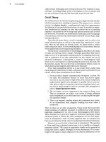
I/ASSESSMENT
PROBLEMS
Objective 1—Know the RL and RC circuit configurations that act as low-pass filters
14.1 A series RC low-pass filter requires a cutoff
frequency of 8 kHz. Use R = 10 kfl and com-
pute the value of C required.
Answer: 1.99 nF.
NOTE: Also try ChapterProblems 14.1 and 14.2.
14.2 A series RL low-pass filter with a cutoff fre-
quency of 2 kHz is needed. Using R = 5 kft,

compute (a) L; (b) \H(joi)\ at 50 kHz; and
(c)
8(ja>)
at 50 kHz.
Answer: (a) 0.40 H;
(b) 0.04;
(c) -87.71°.
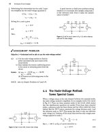
14.3 High-Pass Filters
We next examine two circuits that function as high-pass filters. Once
again, they are the series RL circuit and the series RC circuit. We will see
that the same series circuit can act as either a low-pass or a high-pass filter,
depending on where the output voltage is defined. We will also determine
the relationship between the component values and the cutoff frequency
of these filters.
C
R \ o.
(c)
Figure 14.10 • (a) A series
RC
high-pass filter; (b) the
equivalent circuit at
co
= 0; and (c) the equivalent
circuit at a) = oo.
The
Series RC Circuit—Qualitative
Analysis
A series RC circuit is shown in Fig. 14.10(a). In contrast to its low-pass
counterpart in Fig.
14.7,

the output voltage here is defined across the resis-
tor, not the capacitor. Because of this, the effect of the changing capacitive
impedance is different than it was in the low-pass configuration.
At
co
= 0, the capacitor behaves like an open circuit, so there is no
current flowing in the resistor. This is illustrated in the equivalent circuit in
Fig. 14.10(b). In this circuit, there is no voltage across the resistor, and the
circuit filters out the low-frequency source voltage before it reaches the
circuit's output.
As the frequency of the voltage source increases, the impedance of
the capacitor decreases relative to the impedance of the resistor, and the
source voltage is now divided between the capacitor and the resistor. The
output voltage magnitude thus begins to increase.
When the frequency of the source is infinite
(oo
= oo), the capacitor
behaves as a short circuit, and thus there is no voltage across the capacitor.
This is illustrated in the equivalent circuit in Fig. 14.10(c). In this circuit,
the input voltage and output voltage are the same.
The phase angle difference between the source and output voltages
also varies as the frequency of the source changes. For
oo
= co, the output
voltage is the same as the input voltage, so the phase angle difference is
zero.
As the frequency of the source decreases and the impedance of the
capacitor increases, a phase shift is introduced between the voltage and
the current in the capacitor. This creates a phase difference between the
source and output voltages. The phase angle of the output voltage leads

that of the source voltage. When
oo
= 0, this phase angle difference
reaches its maximum of +90°.
14.3 High-Pass Filters 533
Based on our qualitative analysis, we see that when the output is
defined as the voltage across the resistor, the series RC circuit behaves as
a high-pass filter. The components and connections are identical to the
low-pass series RC circuit, but the choice of output is different. Thus, we
have confirmed the earlier observation that the filtering characteristics of
a circuit depend on the definition of the output as well as on circuit com-
ponents, values, and connections.
Figure 14.11 shows the frequency response plot for the series RC
high-pass filter. For reference, the dashed lines indicate the magnitude
plot for an ideal high-pass filter. We now turn to a quantitative analysis of
this same circuit.
The Series
RC
Circuit—Quantitative Analysis
To begin, we construct the ^-domain equivalent of the circuit in
Fig. 14.10(a). This equivalent is shown in Fig. 14.12. Applying s-domain
voltage division to the circuit, we write the transfer function:
H(s)
l«0)|
s + IjRC
Making the substitution s = j(o results in
Figure 14.11 • The frequency response plot for the
series
RC
circuit in Fig. 14.10(a).

H(jo>) =
)<»
jo) + 1/RC
(14.15)
Next, we separate Eq. 14.15 into two equations. The first is the equation
describing the magnitude of the transfer function; the second is the equa-
tion describing the phase angle of the transfer function:
\H(jco)\
=
co
Vcv
2
+ (l/i?C)
2
'
6(jco) = 90° - tan ~
l
cvRC.
(14.16)
(14.17)
A close look at Eqs. 14.16 and 14.17 confirms the shape of the frequency
response plot in Fig.
14.11.
Using Eq. 14.16, we can calculate the cutoff fre-
quency for the series RC high-pass filter. Recall that at the cutoff frequency,
the magnitude of the transfer function is (1/V2)//
max
. For a high-pass filter,
#max
=

l#(yw)|
w
=oo = \H(joo)\, as seen from Fig.
14.11.
We can construct
an equation for (o
c
by setting the left-hand side of Eq. 14.16 to
(l/y/2)\H(joo)\, noting that for this series RC circuit, \H(joo)\ = 1:
J_
sC
Vi(s)
+
Figure 14.12 A The s-domain equivalent of the circuit
in Fig. 14.10(a).
1
co,
V2 Vco? + (l/RC)
2
(14.18)
Solving Eq. 14.18 for
o)
c
,
we get
1
RC
(14.19)
Equation 14.19 presents a familiar result. The cutoff frequency for the
series RC circuit has the value l/RC, whether the circuit is configured as a

low-pass filter in Fig. 14.7 or as a high-pass filter in Fig. 14.10(a). This is
perhaps not a surprising result, as we have already discovered a connec-
tion between the cutoff frequency,
co
c
,
and the time constant,
T,
of a circuit.
Example 14.3 analyzes a series RL circuit, this time configured as a
high-pass filter. Example 14.4 examines the effect of adding a load resistor
in parallel with the inductor.
534 Introduction to Frequency Selective Circuits
Example 14.3
Designing a Series
RL
High-Pass Filter
Show that the series RL circuit in Fig. 14.13 also
acts like a high-pass filter:
a) Derive an expression for the circuit's transfer
function.
b) Use the result from (a) to determine an equation
for the cutoff frequency in the series RL circuit.
c) Choose values for R and L that will yield a high-
pass filter with a cutoff frequency of 15 kHz.
Figure 14.14 •
The
s-domain equivalent of
the
circuit in

Fig.
14.13.
Figure 14.13 •
The
circuit for Example 14.3.
Solution
a) Begin by constructing the .v-domain equivalent
of the series RL circuit, as shown in Fig. 14.14.
Then use .v-domain voltage division on the equiv-
alent circuit to construct the transfer function:
H(s) =
s + R/L
Making the substitution s =
ja>,
we get
H(jco) =
jco + R/L'
Notice that this equation has the same form as
Eq. 14.15 for the series RC high-pass filter.
b) To find an equation for the cutoff frequency, first
compute the magnitude of H(jco):
|//{/a,)|
=
CO
Vor +
(R/L)
2
Then, as before, we set the left-hand side of this
equation to (l/V2)//
max

, based on the defini-
tion of the cutoff frequency
co
c
.
Remember that
#max ~ IHQ
00
)1 f°
r a
high-pass filter, and for
the series RL circuit, |//(j'oo)| = 1. We solve the
resulting equation for the cutoff frequency:
1
V2
Vto;
+
(R/L)
2
'
co,
=
R
L
This is the same cutoff frequency we computed
for the series RL low-pass filter.
c) Using the equation for
co
c
computed in (b), we

recognize that it is not possible to specify values
for R and L independently. Therefore, let's arbi-
trarily select a value of 500 O for JR. Remember
to convert the cutoff frequency to radians per
second:
L
R_
CO,.
500
(2TT)(15,000)
5.31 mH.
Example 14.4
Loading the Series RL High-Pass Filter
Examine the effect of placing a load resistor in par-
allel with the inductor in the RL high-pass filter
shown in Fig. 14.15:
a) Determine the transfer function for the circuit in
Fig. 14.15.
b) Sketch the magnitude plot for the loaded RL
high-pass filter, using the values for R and L
from the circuit in Example 14.3(c) and letting
R
L
= R. On the same graph, sketch the magni-
tude plot for the unloaded RL high-pass filter of
Example 14.3(c).
Solution
a) Begin by transforming the circuit in Fig. 14.15 to
the i-domain, as shown in Fig. 14.16. Use voltage
division across the parallel combination of

inductor and load resistor to compute the trans-
fer function:
H(s)
R
L
sL
R
L
+ sL
R,
R + R
L
Ks
R +
R
L
sL
R
r
+ sL
s +
R
L
\R s + to
t
R + RrjL
143 High-Pass Filters 535
where
K =
i?i

R + R
L
'
u>
c
= KR/L.
Note that a)
c
is the cutoff frequency of the
loaded filter.
b) For the unloaded RL high-pass filter from
Example 14.3(c), the passband magnitude is 1,
and the cutoff frequency is 15 kHz. For the
loaded RL high-pass filter, R = R
L
= 500 H, so
K - 1/2. Thus, for the loaded filter, the passband
magnitude is (1)(1/2) = 1/2, and the cutoff fre-
quency is (15,000)(1/2) = 7.5 kHz. A sketch of
the magnitude plots of the loaded and unloaded
circuits is shown in Fig. 14.17.
RL
Figure 14.15 A The circuit for Example 14.4.
Vfa)
Figure 14.16 • The 5-domain equivalent of the circuit in
Fig.
14.15.
0 £.10 /;. 20 30 40 50
Frequency (kHz)
Figure 14.17 • The magnitude plots for the unloaded

RL
high-pass filter of Fig 14.13 and the loaded
RL
high-pass filter
of
Fig.
14.15.
Comparing the transfer functions of the unloaded filter in Example 14.3
and the loaded filter in Example 14.4 is useful at this point. Both transfer
functions are in the form:
H(s) =
Ks
s + K{R/LY
with K = 1 for the unloaded filter and K = R
L
/(R + R
L
) for the loaded
filter. Note that the value of K for the loaded circuit reduces to the value
of K for the unloaded circuit when R
L
= oo; that
is,
when there is no load
resistor. The cutoff frequencies for both filters can be seen directly from
their transfer functions. In both cases,
co
c
= K(R/L), where K = 1 for the
unloaded circuit, and K = RJ{R + RfJ for the loaded circuit. Again, the

cutoff frequency for the loaded circuit reduces to that of the unloaded cir-
cuit when R
L
= oo. Because R
L
/(R + RL) < h the effect of the load
resistor is to reduce the passband magnitude by the factor K and to lower
the cutoff frequency by the same factor. We predicted these results at the
beginning of this chapter. The largest output amplitude a passive high-pass
filter can achieve is 1, and placing a load across the filter, as we did in
Example 14.4, has served to decrease the amplitude. When we need to
amplify signals in the passband, we must turn to active filters, such as those
discussed in Chapter 15.
The effect of a load on a filter's transfer function poses another
dilemma in circuit design. We typically begin with a transfer function spec-
ification and then design a filter to produce that function. We may or may
not know what the load on the filter will be, but in any event, we usually
want the filter's transfer function to remain the same regardless of the
load on it. This desired behavior cannot be achieved with the passive fil-
ters presented in this chapter.
ff(s)
H(s)
s
s + R/L
R/L
Figure 14.18 • Two high-pass filters, the series
RC
and
the series
RL,

together with their transfer functions and
cutoff frequencies.