Electric Circuits, 9th Edition P64 doc

606 Fourier Series
4) + 27/
Figure 16.1 A A periodic waveform.
v{t)
V
m
-
v(t)
V,„ -
T
(a)
27
7/2
(b)
Figure 16.2 • Output waveforms of
a
nonfiltered
sinu-
soidal rectifier, (a) Full-wave rectification, (b) Half-wave
rectification.
Another practical problem that stimulates interest in periodic func-
tions is that power generators, although designed to produce a sinusoidal
waveform, cannot in practice be made to produce a pure sine wave. The
distorted sinusoidal wave, however, is periodic. Engineers naturally are
interested in ascertaining the consequences of exciting power systems
with a slightly distorted sinusoidal voltage.
Interest in periodic functions also stems from the general observation
that any nonlinearity in an otherwise linear circuit creates a nonsinusoidal
periodic function. The rectifier circuit alluded to earlier is one example of
this phenomenon. Magnetic saturation, which occurs in both machines
and transformers, is another example of a nonlinearity that generates a

nonsinusoidal periodic function. An electronic clipping circuit, which uses
transistor saturation, is yet another example.
Moreover, nonsinusoidal periodic functions are important in the
analysis of nonelectrical systems. Problems involving mechanical vibra-
tion, fluid flow, and heat flow all make use of periodic functions. In fact,
the study and analysis of heat flow in a metal rod led the French mathe-
matician Jean Baptiste Joseph Fourier (1768-1830) to the trigonometric
series representation of a periodic function. This series bears his name and
is the starting point for finding the steady-state response to periodic exci-
tations of electric circuits.
V
m
-
Figure 16.3 A The triangular waveform of
a
cathode-ray
oscilloscope sweep generator.
v(t)
Vm
0
1/
v
m n
7
27
(a)
V(
Vm
0
0

r
2 7
(c)
Figure 16.4 A Waveforms produced by function
generators used in laboratory testing, (a) Square wave,
(b) Triangular wave, (c) Rectangular pulse.
16.1 Fourier Series Analysis:
An
Overview
607
16.1 Fourier Series Analysis:
An Overview
What Fourier discovered in investigating heat-flow problems is that a
periodic function can be represented by an infinite sum of sine or cosine
functions that are harmonically related. In other words, the period of any
trigonometric term in the infinite series is an integral multiple, or har-
monic, of the fundamental period T of the periodic function. Thus for peri-
odic /(/), Fourier showed that /(/) can be expressed as
oo
f(t) = a
v
+ 5X
cos n(a
d
+ b
n sin/iwo^ (16.2) < Fourier series representation of a periodic
«=i function
where n is the integer sequence 1,2,3,
In Eq.
16.2,

a
v
, a
fn
and b
n
are known as the Fourier coefficients and are
calculated from /(f). The term o>
0
(which equals
2TT/T)
represents the
fundamental frequency of the periodic function /(f). The integral multi-
ples of
OJ
()
—that is,
2&>
0
,
3a>
0
, 4w
0
, and so on—are known as the harmonic
frequencies of/(/). Thus 2w
0
is the second harmonic, 3a>
0
is the third har-

monic, and
no)
()
is the «th harmonic of /(f).
We discuss the determination of the Fourier coefficients in
Section 16.2. Before pursuing the details of using a Fourier series in circuit
analysis, we first need to look at the process in general terms. From an
applications point of view, we can express all the periodic functions of
interest in terms of a Fourier series. Mathematically, the conditions on a
periodic function /(f) that ensure expressing /(f) as a convergent Fourier
series (known as Dirichlet's conditions) are that
1.
/(f) be single-valued,
2.
/(/) have a finite number of discontinuities in the periodic interval,
3.
/(/) have a finite number of maxima and minima in the periodic
interval,
4.
the integral
/
1/(01*
exists.
Any periodic function generated by a physically realizable source satisfies
Dirichlet's conditions. These are sufficient conditions, not necessary con-
ditions. Thus if /(f) meets these requirements, we know that we can
express it as a Fourier series. However, if/(f) docs not meet these require-
ments, we still may be able to express it as a Fourier series. The necessary
conditions on /(f) are not known.
After we have determined /(f) and calculated the Fourier coefficients

(«,„
a,„
and b„), we resolve the periodic source into a dc source (a„) plus a
sum of sinusoidal sources
(a„
and /?„). Because the periodic source is driv-
ing a linear circuit, we may use the principle of superposition to find the
steady-state response. In particular, we first calculate the response to each
source generated by the Fourier series representation of/(f) and then add
the individual responses to obtain the total response. The steady-state
response owing to a specific sinusoidal source is most easily found with
the phasor method of analysis.
The procedure is straightforward and involves no new techniques of
circuit analysis. It produces the Fourier series representation of the
steady-state response; consequently, the actual shape of the response is
608 Fourier Series
unknown. Furthermore, the response waveform can be estimated only by
adding a sufficient number of terms together. Even though the Fourier
series approach to finding the steady-state response does have some draw-
backs,
it introduces a way of thinking about a problem that is as important
as getting quantitative results. In fact, the conceptual picture is even more
important in some respects than the quantitative one.
16.2 The Fourier Coefficients
After defining a periodic function over its fundamental period, we deter-
mine the Fourier coefficients from the relationships
a
v
= f.
/(

?
)
dt
>
(
16
-
3
)
2 /
Fourier coefficients • a
k
= —I f(t) cos kco
0
t dt, (16.4)
Tj
t(3
2 f'o+T
b
k = r fit) sin
ka)
Q
t
dt. (16.5)
1
J t
0
In Eqs. 16.4 and 16.5, the subscript k indicates the &th coefficient in the
integer sequence 1,2,3, Note that a
v

is the average value of
/(/),
a
k
is
twice the average value of f{t) cos
kcotf,
and b
k
is twice the average value
of f(t) sin
kcotf.
We easily derive Eqs. 16.3-16.5 from Eq. 16.2 by recalling the follow-
ing integral relationships, which hold when m and n are integers:
sin mw
0
f dt = 0, for all m, (16.6)
'o
t
0
+T
cos mcootdt
= 0, for all m, (16-7)
I
Jtr,
t
n
+T
cos
moitf

sin
nco^t
dt = 0, for all m and n, (16.8)
t
0
+r
sin
mo)()t
sin
no)
{)
t
dt = 0, for all m # n,
= —, for m - n, (16.9)
2
to+T
cos mo)
0
t
cos
nco
G
t
dt = 0, for all m # «,
T
= —, for m = n. (16.10)
We leave you to verify
Eqs.
16.6-16.10 in Problem 16.5.
16.2 The Fourier Coefficients 609

To derive Eq. 16.3, we simply integrate both sides of Eq. 16.2 over
one period:
rt
{)
+T rh+T / oo \
/ f(t)dt = / f a
v
4- ^ a
n
cos
n(x)
()
t
+ b
lt
sinna)
{)
t jdt
Jio Ji,) \ «=l /
/.?„+'/'
oo rh+T
= / a
v
dt + 2 / (
fl
«
cos
nw
o*
+

^«
sm
'""of) &
J/
tl
11=
1
Jfy
a
v
T + 0.
(16.11)
Equation 16.3 follows directly from Eq.
16.11.
To derive the expression for the A:th value of
A„,
we first multiply
Eq. 16.2 by cos kio
{)
t and then integrate both sides over one period of /(f):
f„+r
,-tu+T
f{t)
cos kco
{)
t
dt = / a
v
cos k(o
{)

t
dt
+
2)/
(«/,
cos
«o>
(
/
cos &w
()
f
+
/}„ sin
«6>
(
/
cos /ca>
()
f)
d/
«=1 A,
'«
= 0 + a
A
|y)
(16.12)
Solving Eq. 16.12 for a
k
yields the expression in Eq. 16.4.

We obtain the expression for the
kXh.
value of b
n
by first multiplying
both sides of Eq. 16.2 by sin kcotf and then integrating each side over one
period of/(f). Example 16.1 shows how to use Eqs. 16.3-16.5 to find the
Fourier coefficients for a specific periodic function.
Example 16.1
Finding the Fourier Series of a Triangular Waveform with No Symmetry
Find the Fourier series for the periodic voltage
shown in Fig. 16.5.
-7 0 T IT
Figure 16.5 •
The
periodic voltage for Example 16.1.
Solution
When using Eqs. 16.3-16.5 to find a
v
, %, and b
k
, we
may choose the value of f
0
-
FOT
the periodic voltage
of Fig. 16.5, the best choice for f
()
is zero. Any other

choice makes the required integrations more cum-
bersome. The expression for v(t) between 0 and 7 is
ly
1
The equation for a
v
is
1
f
T
fV
a
-
=
H
KTr
=
i
v
'
This is clearly the average value of the waveform in
Fig. 16.5.
The equation for the kth value of a
n
is
(lk
=
T
I
1*7^

'
2V
1
*
•Z—z COS k(Ont + ~ SmkiOnt
T
2
Kk
2
^ kc*a
2V,
T
2
——z ( cos
2-rrk
- 1) 0 for all k.
610 Fourier Series
The equation for the A:th value of
b„
is
bk =
T
I
\^r
L
)
tsinko)[)tdt
2V
"'f
l

i
t
i \
T
o
2V
m
( T \
=
0
0 , coslirk
T
2
\ kcou J
-v
m
irk
y
m
=
— -
y
y
m
2
The Fourier series for v(t) is
V °9 1
v
in ^r\
l

.
X~ smtt&w
K V V
sm
(o
{)
t
- -— sin
2oj
()
t
-
——
sin
3a>
0
?
-
• •
•.
1" 27T 37T
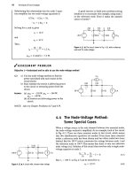
I/ASSESSMENT
PROBLEMS
Objective 1—Be able to calculate the trigonometric form of the Fourier coefficients for a periodic waveform
16.1 Derive the expressions for «„, a
k
, and b
k
for the
periodic voltage function shown if V

m
= 9ir V.
v„
3
27/
3
4T
3
57/
3
IT
f sin^ V,
Answer: a
v
= 21.99 V,
NOTE: Also try Chapter Problems 16.1-16.3.
cos^) V.
16.2 Refer to Assessment Problem 16.1.
a) What is the average value of the periodic
voltage?
b) Compute the numerical values of
ay
— a
5
and b\ - b
5
.
c) If T = 125.66 ms, what is the fundamental
frequency in radians per second?
d) What is the frequency of the third harmonic

in hertz?
e) Write the Fourier series up to and including
the fifth harmonic.
Answer: (a) 21.99 V;
(b) -5.2 V,2.6V,0V,-1.3, and 1.04 V;
9
V, 4.5 V,
0
V,
2.25
V,
and 1.8 V;
(c) 50 rad/s;
(d) 23.87 Hz;
(e) v(t) = 21.99 - 5.2 cos
50?
+
9
sin
50?
+
2.6 cos 100? + 4.5 sin
100*
-
1.3 cos 200? + 2.25 sin 200? +
1.04 cos 250? + 1.8 sin 250? V.
Finding the Fourier coefficients, in general, is tedious. Therefore any-
thing that simplifies the task is beneficial. Fortunately, a periodic function
that possesses certain types of symmetry greatly reduces the amount of
work involved in finding the coefficients. In Section 16.3, we discuss how

symmetry affects the coefficients in a Fourier series.
16.3 The Effect of Symmetry on the Fourier Coefficients 611
16.3 The Effect of Symmetry
on the Fourier Coefficients
Four types of symmetry may be used to simplify the task of evaluating the
Fourier coefficients:
• even-function symmetry,
• odd-function symmetry,
• half-wave symmetry,
• quarter-wave symmetry.
The effect of each type of symmetry on the Fourier coefficients
is
discussed
in the following sections.
Even-Function Symmetry
A function is defined as even if
fit) = /(-0-
(16.13)
-<
Even function
Functions that satisfy Eq. 16.13 are said to be even because polynomial
functions with only even exponents possess this characteristic. For even
periodic functions, the equations for the Fourier coefficients reduce to
2
f
T/2
(16.14)
T/2
f{t) cos ktotfdt,
1

Jo
(16.15)
b
k
= 0, for all k.
(16.16)
Note that all the b coefficients are zero if the periodic function is even.
Figure 16.6 illustrates an even periodic function. The derivations of
Eqs.
16.14-16.16 follow directly from Eqs. 16.3-16.5. In each derivation,
we select t
{)
= -T/2 and then break the interval of integration into the
range from -T/2 to 0 and 0 to T/2, or
a
r
-T/2
-T/2
0
/(0 dt
T/2
T/2
"fl
f(t)dL
(16.17)
-T
m
0
Figure 16.6 • An even periodic function,
/(0=/(-0-

Now we change the variable of integration in the first integral on the
right-hand side of Eq. 16.17. Specifically, we let t = -x and note that
/(0
=
f(~
x
)
=
/(•*) because the function is even. We also observe that
x
—
T/2 when t = -T/2 and dt =
—dx.
Then
/(0 dt -
T/2 J'T/2
0 /-7/2
f(x)(-dx) = / f(x) dx, (16.18)
612 Fourier Series
which shows that the integration from -T/2 to 0 is identical to that from
0 to 7/2; therefore Eq. 16.17 is the same as Eq. 16.14. The derivation of
Eq. 16.15 proceeds along similar lines. Here,
a
k
=
2
f°
/(/) cos
ka)
{)

t
dt
T/2
V — / /(/) cos
ko)
{)
t
dt,
' h)
(16.19)
but
•4) ,.()
/(/) cos
ku>()tdt
= / f(x) cos (-k00^)(-dx)
T/2 JT/2
T/2
f(x) cos
k(x)
{)
x
dx.
(16.20)
As before, the integration from -T/2 to 0 is identical to that from 0 to
T/2. Combining Eq. 16.20 with Eq. 16.19 yields Eq. 16.15.
All the b coefficients are zero when /(/) is an even periodic function,
because the integration from —T/2 to 0 is the exact negative of the inte-
gration from 0 to T/2; that is,
0 ni)
/(/) sin

ka)
{)
t
dt = / f(x)sm(-ko)
{)
x)(—dx)
-T/2 JT/2
T/2
f(x) sin
koi()X
dx. (16.21)
When we use Eqs. 16.14 and 16.15 to find the Fourier coefficients, the
interval of integration must be between 0 and T/2.
Odd-Function Symmetry
A function is defined as odd if
Odd function •
Figure 16.7 •
An
odd periodic function
/(0 =
-/(-0.
m
=
-/(-0.
(16.22)
Functions that satisfy Eq. 16.22 are said to be odd because polynomial
functions with only odd exponents have this characteristic. The expres-
sions for the Fourier coefficients are
a
v

= 0;
a
k
= 0,
6
*
=
f
for all k\
rT/2
/ /(/) sin
ka)
{)
t
dt.
/o
(16.23)
(16.24)
(16.25)
Note that all the a coefficients are zero if the periodic function is odd.
Figure 16.7 shows an odd periodic function.
16.3
The
Effect
of
Symmetry on
the
Fourier Coefficients
613
We

use the
same process
to
derive
Eqs.
16.23-16.25 that
we
used
to
derive
Eqs.
16.14-16.16.
We
leave
the
derivations
to
you
in
Problem
16.7.
The evenness,
or
oddness,
of a
periodic function
can be
destroyed
by
shifting

the
function along
the
time axis.
In
other words,
the
judicious
choice
of
where
t - 0
may
give
a
periodic function even
or
odd
symmetry.
For example,
the
triangular function shown
in
Fig.
16.8(a)
is
neither even
nor
odd.
However,

we can
make
the
function even,
as
shown
in
Fig. 16.8(b),
or
odd, as
shown
in
Fig.
16.8(c).
Half-Wave Symmetry
A periodic function possesses half-wave symmetry
if it
satisfies
the
constraint
/(f)
= -f(t - T/2).
(16.26)
Equation
16.26
states that
a
periodic function
has
half-wave symmetry

if,
after
it is
shifted one-half period
and
inverted,
it is
identical
to
the
original
function.
For
example,
the
functions shown
in
Figs.
16.7
and
16.8
have
half-
wave symmetry, whereas those
in
Figs. 16.5
and
16.6
do
not.

Note that
half-
wave symmetry
is
not
a
function
of
where
t = 0.
If
a
periodic function
has
half-wave symmetry, both
a
k
and
b
k
are
zero
for even values
of k.
Moreover,
a
v
also
is
zero because

the
average value
of
a
function with half-wave symmetry
is
zero.
The
expressions
for the
Fourier coefficients
are
a
v
= 0,
a
k
= 0,
(16.27)
7/2
1
-/()
h =
o,
h
= y7
T/2
fit) cos
ko)
0

t
dt,
i
fit) sin
k(i)
{)
t
dt,
for
k
even;
for
k
odd;
for
k
even;
for
k
odd.
(16.28)
(16.29)
(16.30)
(16.31)
(c)
Figure
16.8
A
How the choice
of

where
t = 0
can
make
a
periodic function even, odd,
or
neither,
(a) A
periodic triangular wave that
is
neither even
nor
odd.
(b) The triangular wave
of
(a)
made even
by
shifting
the
function along
the
t
axis,
(c)
The triangular wave
of
(a)
made odd

by
shifting
the
function along
the
t
axis.
We derive
Eqs.
16.27-16.31
by
starting with
Eqs.
16.3-16.5
and
choos-
ing
the
interval
of
integration
as
—T/2
to T/2. We
then divide this range
into
the
intervals
—T/2 to 0 and 0 to T/2. For
example,

the
derivation
for
a
k
is
a
k
=
Jt,
t
fit)
cos
kcjQt
dt
T.L
T/2
fit)
cos
kco
{)
t
dt
T
L
T/2
.0
=
— / fit)
cos

kcoot
dt
T/2
T/2
+
;=r / /(f)
cos
ka)
{]
t
dt.
'
-A)
(16.32)
614 Fourier Series
Now we change a variable in the first integral on the right-hand side of
Eq. 16.32. Specifically, we let
Then
t = x - T/2.
x = T/2, when t = 0;
x = 0, when t = —T/2;
dt = dx.
We rewrite the first integral as
/(0 cos kto
()
tdt =/ f(x - T/2)coskto
{)
(x -
T/2)dx.
(16.33)

-T/2
Ml
Note that
cos
ktO()(x —
T/2) — cos (ko)
{)
x — kir) = cos kir cos
kco
()
x
and that, by hypothesis,
f(x - T/2) =
-f(x).
Therefore Eq. 16.33 becomes
A
7/4
-A
7/2 37/4 7
(a)
/(0
/I
0
-
i
7/4
-A
I
7/2 37/4
7

(b)
Figure 16.9 • (a) A function that has quarter-wave
symmetry, (b) A function that does not have quarter-
wave symmetry.
./-7/2
f(t) cos
kco
()
t
dt
T/2
[-f(x)] cos k
77
cos ko)
{)
x dx. (16.34)
t
Incorporating Eq. 16.34 into Eq. 16.32 gives
7/2
a
k
= -(1
—
cos kit) / f(t) cos &G>
0
f rf/.
(16.35)
But cos
kTT
is 1 when k is even and -1 when k is odd. Therefore Eq. 16.35

generates Eqs. 16.28 and 16.29.
We leave it to you to verify that this same process can be used to
derive Eqs. 16.30 and 16.31 (see Problem 16.8).
We summarize our observations by noting that the Fourier series rep-
resentation of a periodic function with half-wave symmetry has zero aver-
age,
or dc, value and contains only odd harmonics.
Quarter-Wave Symmetry
The term quarter-wave symmetry describes a periodic function that has
half-wave symmetry and, in addition, symmetry about the midpoint of the
positive and negative half-cycles. The function illustrated in Fig. 16.9(a)
16.3 The Effect of Symmetry on the Fourier Coefficients 615
has quarter-wave symmetry about the midpoint of the positive and nega-
tive half-cycles. The function in Fig. 16.9(b) does not have quarter-wave
symmetry, although it does have half-wave symmetry.
A periodic function that has quarter-wave symmetry can always be
made either even or odd by the proper choice of the point where t = 0.
For example, the function shown in Fig. 16.9(a) is odd and can be made
even by shifting the function 7/4 units either right or left along the t axis.
However, the function in Fig. 16.9(b) can never be made either even or
odd. To take advantage of quarter-wave symmetry in the calculation of the
Fourier coefficients, you must choose the point where t = 0 to make the
function either even or odd.
If the function is made even, then
a
v
= 0, because of half-wave symmetry;
a
k
= 0, for k even, because of half-wave symmetry;

8
f
T/4
a
k
= — I f(t) cos kaitf dt, for k odd;
T Ju
b
k
= 0, for all /c, because the function is even. (16.36)
Equations 16.36 result from the function's quarter-wave symmetry in
addition to its being even. Recall that quarter-wave symmetry is super-
imposed on half-wave symmetry, so we can eliminate a
r
and a
k
for k even.
Comparing the expression for a
k
, k odd, in Eqs. 16.36 with Eq. 16.29 shows
that combining quarter-wave symmetry with evenness allows the shorten-
ing of the range of integration from 0 to 7/2 to 0 to 7/4. We leave the der-
ivation of Eqs. 16.36 to you in Problem 16.9.
If the quarter-wave symmetric function is made odd,
a
v
= 0, because the function is odd;
a
k
= 0, for all k, because the function is odd;

b
k
= 0, for k even, because of half-wave symmetry;
8
f
T/4
b
k = ^ / f(t) sin kco
{)
tdt, for k odd. (16.37)
Equations 16.37 are a direct consequence of quarter-wave symmetry and
oddness. Again, quarter-wave symmetry allows the shortening of the inter-
val of integration from 0 to 7/2 to 0 to 7/4. We leave the derivation of
Eqs.
16.37 to you in Problem 16.10.
Example 16.2 shows how to use symmetry to simplify the task of find-
ing the Fourier coefficients.