Electric Circuits, 9th Edition P65 pptx

616 Fourier Series
Example 16.2
Finding the Fourier Series of an Odd Function with Symmetry
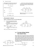
Find the Fourier series representation for the cur-
rent waveform shown in Fig, 16.10.
-T/2
Figure 16.10 •
The
periodic waveform for Example 16.2.
In the interval Ost < 7/4, the expression for
/(f) is
m-f,
Thus
8
f
T/4
4I
b
k
= — —risinkaitfdt
1
Jo *
321
m
I sin ktoot t cos
kco
()
t
2 2
T
l

\ kW
0
k(0()
TfA
Solution
We begin by looking for degrees of symmetry in the
waveform. We find that the function is odd and, in
addition, has half-wave and quarter-wave symme-
try. Because the function is odd, all the a coeffi-
cients are zero; that is, a
v
= 0 and a
k
= 0 for all k.
Because the function has half-wave symmetry,
b
k
= 0 for even values of k. Because the function
has quarter-wave symmetry, the expression for b
k
for odd values of k is
8j,
/« . kir
2 7
sin — {k is odd).
Kr £
TT
The Fourier series representation of /(f) is
i(t)
=—r*

2J ~ sin —- sin «<W
0
/
TT"
«
=
1,3.5, «
2
—r sin
w
Q
t
- - sin
3<o
G
t
IT
1
V y
r/4
b
k
=-= f /(f) sin
ko)
{]
t
dt.
1
-A)
+ — sm Statf - — sin 7^ +

/ASSESSMENT
PROBLEM
Objective 1—Be able to calculate the trigonometric form of the Fourier coefficients for a periodic waveform
16.3 Derive the Fourier series for the periodic volt-
age shown.
\7V
m
« sin (mr/3) .
Answer: v
g
(t) = —z— 2J z smnco
0
t.
TT
«=1,3,5, n
MO
v
m
-v
m
/ \ 1 \
0 T/6 T/3 r/s
—
1 1
.27/3
57/6
/
/T
NOTE: Also try Chapter Problems 16.11 and 16.12.
16.4 An Alternative Trigonometric Form of the Fourier Series 617

16.4 An Alternative Trigonometric Form
of the Fourier Series
In circuit applications of the Fourier series, we combine the cosine and
sine terms in the series into a single term for convenience. Doing so allows
the representation of each harmonic of v(t) or i(t) as a single phasor quan-
tity. The cosine and sine terms may be merged in either a cosine expres-
sion or a sine expression. Because we chose the cosine format in the
phasor method of analysis (see Chapter 9), we choose the cosine expres-
sion here for the alternative form of the series. Thus we write the Fourier
series in Eq. 16.2 as
fit) = a
v
+ ^A
n
cos(no)
{)
t - 6,X (16.38)
«=i
where A
n
and
d„
are defined by the complex quantity
a
n
- jb
n
= Vflg + bl/-6
n
=

A
a
/-9„.
(16.39)
We derive Eqs. 16.38 and 16.39 using the phasor method to add the cosine
and sine terms in Eq. 16.2. We begin by expressing the sine functions as
cosine functions; that is, we rewrite Eq. 16.2 as
00
/(/) = a
v
+ 2X,cosncotf + b
n
cos(nco
0
t - 90°). (16.40)
Adding the terms under the summation sign by using phasors gives
SP{fl„ cos natf} = a
n
/0^ (16.41)
and
®{b„
cos(nco
()
t
- 90°)} = b
n
/-90° = -jb
n
. (16.42)
Then

2P{«„ cos(«a>o* + b
n
cos(ti(OQt
— 90°)} = a
n
- jb
n
= Val
+
%/-$„
=
A„/-0„.
(16.43)
When we inverse-transform Eq.
16.43,
we get
a
n
cosno)
()
t + b
n
cos(nw
0
t - 90°) = ^jA,,/-6,,}
= A
n
cos(no)
0
t - 6

n
). (16.44)
Substituting Eq. 16.44 into Eq. 16.40 yields Eq. 16.38. Equation 16.43
corresponds to Eq. 16.39. If the periodic function is either even or odd,
A
n
reduces to either a
n
(even) or
b„
(odd), and 6
n
is either 0° (even) or
90° (odd).
The derivation of the alternative form of the Fourier series for a given
periodic function is illustrated in Example 16.3.
618 Fourier Series
Example 16.3
Calculating Forms of the Trigonometric Fourier Series for Periodic Voltage
a) Derive the expressions for a
k
and b
k
for the peri-
odic function shown in Fig.
16.11.
b) Write the first four terms of the Fourier series
representation of v(t) using the format of
Eq. 16.38.
J L

T_ T_ yr T 5T 3T IT 2T
4 2 4 4 2 4
Figure 16.11 • The periodic function for Example 16.3.
Solution
a) The voltage v(t) is neither even nor odd, nor
does it have half-wave symmetry. Therefore we
use Eqs. 16.4 and 16.5 to find a
k
and b
k
. Choosing
to as zero, we obtain
a
k
=
T
7*/4 PT
V
m
cos ko)
{)
t dt + (0) cos
ka>
{)
t
dt
JTjA
2V
m
smkcotf

kcor
7/4
0
Vjn . kTJ^
kir 2
and
2 [
T/A
b
k
= — I V
m
sin ktntf dt
1
Jo
2V
m
( — cos koot
k(o
{)
V
m
(. k-n•
b) Tlie average value of v{t) is
a„ = -— = -v
The values of a
k
— jb
k
for k = 1,2, and 3 are

«i - jb\
V,
IT
V,
TT
V2V,
/-45°,
V V
(h —
lb~>
= 0 - / = / —90 ,
3
"
J
IT TT
L
«3
_
jb
3
=
-y,>
3TT
Vzv,
3ir
/-135'
Thus the first four terms in the Fourier series
representation of v(t) are
V V2V V
v(t) =^r + -—^-cos^t - 45°) + -f-cos(2co

()
t - 90°)
7T 77
V2V
+ ——^cos(3o>o* - 135°) +
3TT
V U
f
/ASSESSMENT PROBLEM
Objective 1—Be able to calculate the trigonometric form of the Fourier coeffiaents for a periodic waveform
16.4 a) Compute
A\—A
5
and 0i~0
5
for the periodic
function shown if V
m
—
9TT
V.
b) Using the format of Eq. 16.38, write the
Fourier series for v(t) up to and including
the fifth harmonic assuming T = 125.66 ms.
Answer: (a) 10.4,5.2,0,2.6,2.1 V, and -120°, -60°,
not defined, -120°, -60°;
(b) v(t) = 21.99 + 10.4cos(50/ - 120°) +
5.2cos(100r - 60°) +
2.6 cos(200f - 120°) +
2.1 cos(250/ - 60°) V.

3
IT
3
4J
3
57'
3
IT
NOTE: Also try Chapter Problem 16.22.
16.5 An Application
Now we illustrate how to use a Fourier series representation of a periodic
excitation function to find the steady-state response of a linear circuit. The
RC circuit shown in Fig. 16.12(a) will provide our example. The circuit is
energized with the periodic square-wave voltage shown in Fig. 16.12(b).
The voltage across the capacitor is the desired response, or output, signal.
The first step in finding the steady-state response is to represent the peri-
odic excitation source with its Fourier
series.
After noting that the source has
odd, half-wave, and quarter-wave symmetry, we know that the Fourier
coefficients reduce to b
k
, with k restricted to odd integer values:
b.
T
4V
rrk
774
V
m

sin kaj
{]
t dt
(k is odd).
Then the Fourier series representation of
v„
is
4V
IT
CO -t
- j?
—
sin
nco
{)
t.
(16.45)
(16.46)
Writing the series in expanded form, we have
4K„,
. 4V
m
v., = sin
cunt
+ —— sin 3oW
8
TT 3ir ^
16.5 An Application
(a)
v„

-V,
27 37
(b)
Figure 16.12 A An
RC
circuit excited by a periodic
voltage, (a) The
RC
series circuit, (b) The square-wave
voltage.
4V 4V
in • c ^
v
in • *7 .,
—— sin
5(ti
{)
t
+ —— sin
7ct>
0
/
+
5 7T
777
(16.47)
Tlie voltage source expressed by Eq. 16.47 is the equivalent of infi-
nitely many series-connected sinusoidal sources, each source having its
own amplitude and frequency. To find the contribution of each source to
the output voltage, we use the principle of superposition.

For any one of the sinusoidal sources, the phasor-domain expression
for the output voltage is
V
r
v„ =
1 + jo)RC
(16.48)
All the voltage sources are expressed as sine functions, so we interpret a
phasor in terms of the sine instead of the cosine. In other words, when we
go from the phasor domain back to the time domain, we simply write the
time-domain expressions as sin(atf + 6) instead of cos(wf + 6).
The phasor output voltage owing to the fundamental frequency of the
sinusoidal source is
V,„
=
{4V
m
/ir)/Qf
Writing V„i in polar form gives
cii
where
1 + j(ti
{)
RC '
(4VJ/-/3,
TrVl + (tilR
2
C
r
0i = tan~

X
(ti
{)
RC.
(16.49)
(16.50)
(16.51)
From
Eq.
16.50,
the
time-domain expression
for the
fundamental fre-
quency component
of
v
(
,
is
4V
sin(ttiof
- ft).
(16.52)
TTVI
+ (4RC
2
We derive
the
third-harmonic component

of the
output voltage
in a
simi-
lar manner. The third-harmonic phasor voltage
is
(4V„
;
/377)/cy
Y
"
3
J3(OQRC
4V
f=Zz&> (16.53)
3TTVI
+ 9<4R
2
C
where
j3
3
=
tan~
l
3(o
i}
RC. (16.54)
The time-domain expression
for the

third-harmonic output voltage
is
4V
V
0
3 = , '" = =
=sin(3<o
0
f
- j8
3
).
(16.55)
3TT
VI
+
9wg^
2
C
2
Hence
the
expression
for the
&th-harmonic component
of the
output
voltage
is
v

ok
= '" =
sin(/cw,/
-
j8jt) (&
is
odd), (16.56)
where
/3*
= tan
~
]
k(o
{)
RC
(k is
odd). (16.57)
We
now
write down
the
Fourier series representation
of the
output
voltage:
y
«(0
= ^T 2; / =?•
(16.58)
ff

/, = ul tt VI
+
(HW
0
i?C)
2
The derivation
of
Eq. 16.58 was
not
difficult. But, although we have
an
ana-
lytic expression for the steady-state output, what
v
0
(t)
looks like is not imme-
diately apparent from Eq.
16.58.
As we mentioned earlier, this shortcoming is
a problem with
the
Fourier series approach. Equation 16.58
is not
useless,
however, because
it
gives some feel
for

the steady-state waveform
of
v
(>
(t),
if
we focus
on the
frequency response
of
the circuit. For example,
if C
is large,
1/ncooC
is small
for
the higher order harmonics. Thus the capacitor short cir-
cuits
the
high-frequency components
of
the input waveform,
and the
higher
order harmonics
in
Eq. 16.58 are negligible compared to the lower order har-
monics. Equation 16.58 reflects this condition in that,
for
large

C,
4V
m
°° 1
v
<>
~ S^ 2
-^sin(Aio)
0
r
- 90°)
a
~ 2
-jcosnwof.
(16.59)
7T(D()RC
,, = 1¾
It
Equation 16.59 shows that
the
amplitude
of the
harmonic
in the
output
is decreasing
by 1/n
2
,
compared with

1/n for the
input harmonics.
If C is
so large that only
the
fundamental component
is
significant, then
to a
first approximation
~4V
V»{t)
«
;^cosw
()
f,
(16.60)
16.5
An
Application
621
and Fourier analysis tells
us
that
the
square-wave input
is
deformed into
a
sinusoidal output.

Now let's
see
what happens
as C
—>0.
The circuit shows that
v
()
and v
g
are
the
same when
C = 0,
because
the
capacitive branch looks like
an
open circuit
at all
frequencies. Equation
16.58
predicts
the
same result
because,
as C
—>
0,
W

m
* 1 ,
v
(>
= >.
—
smno)
{)
t. (16.61)
But
Eq.
16.61
is
identical
to Eq.
16.46,
and
therefore
v
0
—*
v
g
as C
—*•
0.
Thus
Eq.
16.58 has proven useful because
it

enabled
us to
predict that
the output will
be a
highly distorted replica
of the
input waveform
if C is
large,
and a
reasonable replica
if C is
small.
In
Chapter 13,
we
looked
at
the distortion between
the
input
and
output
in
terms
of
how much mem-
ory
the

system weighting function had.
In the
frequency domain,
we
look
at
the
distortion between
the
steady-state input
and
output
in
terms
of
how
the
amplitude
and
phase
of the
harmonics
are
altered
as
they
are
transmitted through
the
circuit. When

the
network significantly alters
the
amplitude
and
phase relationships among
the
harmonics
at the
output rel-
ative
to
that
at the
input,
the
output
is a
distorted version
of the
input.
Thus,
in the
frequency domain,
we
speak
of
amplitude distortion
and
phase distortion.

For
the
circuit here, amplitude distortion
is
present because
the
ampli-
tudes
of the
input harmonics decrease
as 1/rc,
whereas
the
amplitudes
of
the output harmonics decrease
as
1
1
n
Vl +
(na>
Q
RC)
2
'
This circuit also exhibits phase distortion because
the
phase angle
of

each
input harmonic
is
zero, whereas that
of
the
nth
harmonic
in the
output sig-
nal
is -
tan"
1
ri(o
0
RC.
An Application
of
the Direct Approach
to
the
Steady-State Response
For
the
simple
RC
circuit shown
in
Fig. 16.12(a), we

can
derive
the
expres-
sion
for the
steady-state response without resorting
to the
Fourier series
representation
of the
excitation function. Doing this extra analysis here
adds
to our
understanding
of
the Fourier series approach.
To find
the
steady-state expression
for v
0
by
straightforward circuit
analysis,
we
reason
as
follows. The square-wave excitation function alter-
nates between charging

the
capacitor toward
+V„, and —V
m
.
After
the
circuit reaches steady-state operation, this alternate charging becomes
periodic. We know from
the
analysis
of
the single time-constant
RC
circuit
(Chapter
7)
that
the
response
to
abrupt changes
in the
driving voltage
is
exponential. Thus
the
steady-state waveform
of the
voltage across

the
capacitor
in the
circuit shown
in
Fig. 16.12(a)
is as
shown
in
Fig.
16.13.
The analytic expressions
for
v„{t)
in the
time intervals
0 < t < T/2
and T/2<t<T
are
Vo
= V
m
+ (V, -
VJe^
RC
,
0 < t < T/2;
(16.62)
Vo
= ~V

m
+ (V
2
+ V
m
)e-^™
RC
, T/2 < t < T.
(16.63)
We derive Eqs. 16.62
and
16.63
by
using the methods
of
Chapter 7, as sum-
marized
by Eq.
7.60.
We
obtain
the
values
of V\ and V
2
by
noting from
Eq. 16.62 that
Vl
= V

m
+ (1/, - V
m
)e-
TI2RC
\
(16.64)
Toward +
V.„
Toward + V.
\
\
Toward —V
m
Toward —V.
Figure
16.13 •
The steady-state waveform
of v
0
for the
circuit
in
Fig. 16.12(a).
622 Fourier Series
Small
C
Figure 16.14 •
The
effect of capacitor size on the

steady-state response.
and from Eq. 16.63 that
V
1
= -V
ln
+ (V
2
+
V
m
)e-
T
?
2RC
.
Solving Eqs. 16.64 and 16.65 for V\ and V
2
yields
y, = -y. = —™i L
Substituting Eq. 16.66 into Eqs. 16.62 and 16.63 gives
2V,
V
° "j" j |_
e
-f/2RC
->/
RC
,
0 < t < T/2.

(16.65)
(16.66)
(16.67)
and
•V
m
+
2V,
1
+
e
-r/ac
ff-(y/2)]/RC
F/2 S / =S 7. (16.68)
Equations 16.67 and 16.68 indicate that v
w
(0 has half-wave symmetry
and that therefore the average value of v
0
is
zero.
This result agrees with
the Fourier series solution for the steady-state response —namely, that
because the excitation function has no zero frequency component, the
response can have no such component. Equations 16.67 and 16.68 also
show the effect of changing the size of the capacitor. If C is small, the
exponential functions quickly vanish, v
a
= V
m

between 0 and T/2, and
v
a
= —V
m
between T/2 and T. In other words, v
a
—*
v%
as C
—>
0. If C is
large, the output waveform becomes triangular in shape, as Fig. 16.14
shows. Note that for large C, we may approximate the exponential
terms
e~'
/RC
and
C
,-['-(772)1/KC
by the Hnear terms
j _
(
t
/RC)
and
1 - {[t - (T/2)]/RC}i respectively. Equation 16.59 gives the Fourier
series of this triangular waveform.
Figure 16.14 summarizes the results. The dashed line in Fig. 16.14 is
the input voltage, the solid colored line depicts the output voltage when

C is small, and the solid black line depicts the output voltage when C
is
large.
Finally, we verify that the steady-state response of Eqs. 16.67 and
16.68 is equivalent to the Fourier series solution in Eq.
16.58.
To do so we
simply derive the Fourier series representation of the periodic function
described by Eqs. 16.67 and
16.68.
We have already noted that the periodic
voltage response has half-wave symmetry. Therefore the Fourier series
contains only odd harmonics. For k odd,
«*
=
T!1
( 2V
e'
t/IiC
(y _
ZK
"'
C
;
—
-8RCV,,,
cos
kco
{)
t

dt
T[\ + (kco
{)
RC)
:
(k is odd),
(16.69)
4 ^/ 2V
m
e-l«
c
b
k
= -
J
\V
m
- -
+
e
_
T/2RC
)
4V,
$kco
(
y
m
R
2

C
2
kir T[\ + (kiOuRC)
2
]
(k is odd).
(16.70)
To show that the results obtained from Eqs. 16.69 and 16.70 are consistent
with Eq. 16.58, we must prove that
4V„,
1
Vol +
b
2
k
=
k7T
Vl + (ka>
{)
RC)
2
'
and that
— = ~ko)[)RC.
(16.71)
(16.72)
16.6 Average-Power Calculations with Periodic Functions 623
We leave you to verify Eqs. 16.69-16.72 in Problems 16.23 and 16.24.
Equations 16.71 and 16.72 are used with Eqs. 16.38 and 16.39 to derive the
Fourier series expression in Eq. 16.58; we leave the details to you in

Problem 16.25.
With this illustrative circuit, we showed how to use the Fourier series
in conjunction with the principle of superposition to obtain the steady-
state response to a periodic driving function. Again, the principal short-
coming of the Fourier series approach is the difficulty of ascertaining the
waveform of the response. However, by thinking in terms of a circuit's fre-
quency response, we can deduce a reasonable approximation of the
steady-state response by using a finite number of appropriate terms in the
Fourier series representation. (See Problems 16.27 and 16.29.)
SSESSMENT PROBLEM
Objective 2—Know how to analyze a circuit's response to a periodic waveform
16.5 The periodic triangular-wave voltage seen on
the left is applied to the circuit shown on the
right. Derive the first three nonzero terms in
the Fourier series that represents the steady-
state voltage v
0
if V
m
= 281.25ir
2
mV and the
period of the input voltage is 200-7T ms.
Answer: 2238.83 cos(10; - 5.71°) + 239.46 cos(30/ -
16.70°) + 80.50 cos(50f - 26.57°) + mV
16.6 The periodic square-wave shown on the left is
applied to the circuit shown on the right.
a) Derive the first four nonzero terms in the
Fourier series that represents the steady-
state voltage v

0
if V„, = 210-77 V and the
period of the input voltage is 0.277 ms.
b) Which harmonic dominates the output
voltage? Explain why.
1
i
y,n
0
~v
m
1
T/2
1
T
100
kft
-^vw—
+
100
nF o
a
Answer: (a) 17.5 cos(10,000r + 88.81°) +
26.14cos(30,000^ - 95.36°) +
168cos(50,0000 +
17.32 cos(70,000/ + 98.30°) + V;
(b) The fifth harmonic, at 10,000 rad/s,
because the circuit is a bandpass filter
with a center frequency of 50,000 rad/s
and a quality factor of 10.

10
kH
!20nF
+
20 mH v„
NOTE: Also try Chapter Problems 16.27 and 16.28.
16.6 Average-Power Calculations
with Periodic Functions
If we have the Fourier series representation of the voltage and current at
a pair of terminals in a linear lumped-parameter circuit, we can easily
express the average power at the terminals as a function of the harmonic
voltages and currents. Using the trigonometric form of the Fourier series
expressed in Eq. 16.38, we write the periodic voltage and current at the
terminals of a network as
00
v = V
dc
+ 2Xcos(/io>of -
Q
m
)<
(16.73)
DO
' = 'dc + ^,I
a
COS(na)
{r
t - B
tn
). (16.74)

/(=1
The notation used in Eqs. 16.73 and 16.74 is defined as follows:
V
dc
= the amplitude of the dc voltage component,
V
n
= the amplitude of the nth-harmonic voltage,
Q
vn
- the phase angle of the nth-harmonic voltage,
/
dc
= the amplitude of the dc current component,
/
n
= the amplitude of the nth-harmonic current,
d
in
= the phase angle of the nth-harmonic current.
We assume that the current reference is in the direction of the refer-
ence voltage drop across the terminals (using the passive sign conven-
tion),
so that the instantaneous power at the terminals is w'.The average
power is
j rh+T j ft
tt
+T
P = ~ / P
dt =

T
Vt dL (16
-
75)
1
Jk
1
At
To find the expression for the average power, we substitute Eqs. 16.73 and
16.74 into Eq. 16.75 and integrate. At first glance, this appears to be a for-
midable task, because the product vi requires multiplying two infinite
series.
However, the only terms to survive integration are the products of
voltage and current at the same frequency. A review of Eqs. 16.8-16.10
should convince you of the validity of this observation. Therefore
Eq. 16.75 reduces to
y^dc^dcf
t
0
+T
oo_
i fh+T
v„i„co$(na)
{)
t
- e
m
)
DO
-i ri

n=\
l
Jt
a
X cos(nw
(
/ - B
in
)dt. (16.76)
Now, using the trigonometric identity
1 1
cos a cos
(3
= -cos(a -/3)+
—
cos(a + /3),
we simplify Eq. 16.76 to
1
°° V I
f'
0+T
p = v
dc
/
dc
+ 7S-^r
1
/
I
cos

(0-
-
*bd
1
;i=i
z
A,
+ cos(2nft)
0
f - 6
m
- d
in
)]dt. (16.77)
The second term under the integral sign integrates to zero, so
P = ^
dc
/
dc
+ 2-^cos(0,„ - 0
in
). (16.78)
Equation 16.78 is particularly important because it states that in the case
of an interaction between a periodic voltage and the corresponding periodic
current, the total average power is the sum of the average powers obtained
from the interaction of currents and voltages of the same frequency. Currents
and voltages of different frequencies do not interact to produce average
16.6
Average-Power Calculations with Periodic Functions 625
power. Therefore,

in
average-power calculations involving periodic func-
tions,
the
total average power
is the
superposition
of the
average powers
associated with each harmonic voltage
and
current. Example 16.4 illustrates
the computation
of
average power involving
a
periodic voltage.
Example 16.4
Calculating Average Power for a Circuit with a Periodic Voltage Source
Assume that
the
periodic square-wave voltage
in
Example
16.3 is
applied across
the
terminals
of a
15

H
resistor. The value
of V
m
is
60 V,
and
that
of T
is
5 ms.
a) Write
the
first five nonzero terms
of the
Fourier
series representation
of v(t). Use the
trigono-
metric form given
in Eq.
16.38.
b) Calculate
the
average power associated with
each term
in (a).
c) Calculate
the
total average power delivered

to
the
15 O
resistor.
d) What percentage
of the
total power
is
delivered
by
the
first five terms
of
the Fourier series?
Solution
a) The dc component of v(t) is
(60)(7/4)
T
= 15 V.
From Example 16.3 we have
A
]
= V2 6O/77 = 27.01 V,
0i = 45°,
A
2
=
60/TT
= 19.10 V,
e

2
= 90°,
A
3
= 20
V2/TT
= 9.00 V,
0
3
= 135°,
A
4
= 0,
04
= 0°,
A
5
=
5.40
V,
05
= 45°,
2TT
277(1000)
w
()
=
40077 rad/s.
Thus,
using

the
first five nonzero terms
of the
Fourier series,
17(f)
= 15 +
27.01 cos(40077/
- 45°)
+
19.10COS(800T7/
- 90°)
+
9.00COS(1200T7/
- 135°)
+ 5.40COS(2000T7/
- 45°)
+ V.
b)
The
voltage
is
applied
to the
terminals
of a
resis-
tor,
so we can
find
the

power associated with
each term
as
follows:
15
2
Pdc=
15"
= 15W
'
1 9
2
P
3
=
__
= 2
.
70W
,
1
5.4
2
,, = -__ =
0.97
W.
c)
To
obtain
the

total average power delivered
to
the
15 0
resistor,
we
first calculate
the rms
value
of
v(t):
V =
r
rms
/(60)
2
(774)
T
= V900
= 30 V.
The total average power delivered
to the 15 (1
resistor
is
30
2
,
P
T
= — =

60
W.
d)
The
total power delivered
by the
first five
nonzero terms
is
P
= P
dc
+ P
{
+ P
2
+ P
3
+ P
5
=
55.15
W.
This
is
(55.15/60)(100),
or
91.92%
of
the total.