Electric Circuits, 9th Edition P68 ppt

646 The Fourier Transform
17.1 The Derivation of the
Fourier Transform
We begin the derivation of the Fourier transform, viewed as a limiting case
of a Fourier series, with the exponential form of the series:
00
f(0 = 2 C
n
e»'«»\ (17.1)
n oa
where
1 f
r/2
C
n
= = / f(t)e-'"^ dt. (17.2)
* J-T/2
In Eq. 17.2, we elected to start the integration at t
0
= -7/2.
Allowing the fundamental period T to increase without limit accom-
plishes the transition from a periodic to an aperiodic function. In other
words, if T becomes infinite, the function never repeats itself and hence is
aperiodic. As T increases, the separation between adjacent harmonic fre-
quencies becomes smaller and smaller. In particular,
Aw = {n + 1)0)() -
HWQ
= o>() = —, (17.3)
and as 7 gets larger and larger, the incremental separation
&co
approaches

a differential separation
dxo.
From Eq. 17.3,
1 doj „
T^ZTT"
^
7-
^
00, (17
'
4
)
As the period increases, the frequency moves from being a discrete vari-
able to becoming a continuous variable, or
nco
0
^u) as 7—»oo. (17.5)
In terms of Eq.
17.2,
as the period increases, the Fourier coefficients C„
get smaller. In the limit, C„—»0 as T—> oo. This result makes sense,
because we expect the Fourier coefficients to vanish as the function loses
its periodicity. Note, however, the limiting value of the product C„T; that is,
C„T~*
f(t)e~
jwt
dt asr-*oo. (17.6)
In writing Eq. 17.6 we took advantage of the relationship in Eq. 17.5.
The integral in Eq. 17.6 is the Fourier transform of /(f) and is denoted
/

00
f(t)e-
ja
" dt. (17.7)
00
17.1 The Derivation of
the
Fourier Transform 647
We obtain an explicit expression for the inverse Fourier transform by
investigating the limiting form of Eq. 17.1 as T—»
DO.
We begin by multi-
plying and dividing by T:
/w= f^
c
«
r
)^(f)
(17.8)
As 7*—»oo, the summation approaches integration, C
n
T
—*
F(co),
n<x)
{)
—>
OJ,
and 1/7
—*

dco/2TT.
Thus in the limit, Eq. 17.8 becomes
m
2ir
F{co)e
io)t
dco.
(17.9) -4 Inverse Fourier transform
Equations 17.7 and 17.9 define the Fourier transform. Equation 17.7 trans-
forms the time-domain expression f(t) into its corresponding frequency-
domain expression F(co). Equation 17.9 defines the inverse operation of
transforming F(co) into/(f).
Let's now derive the Fourier transform of the pulse shown in Fig. 17.1.
Note that this pulse corresponds to the periodic voltage in Example 16.6 if
we let T
—*
oo.The Fourier transform of v(t) comes directly from Eq. 17.7:
V(co)
r/2
V
„£->*"
lit
-r/2
(,->">'
= v,
(-jio)
r/2
-r/2
o(t)
-T/2 0 r/2

Figure 17.1 •
A
voltage pulse.
V
m (
n
. • 0)T
—— -2} sin —
-jot \ 2
(17.10)
which can be put in the form of (sin x)/x by multiplying the numerator
and denominator by T.Then,
V(co) = V
m
r
sin COT/2
COT/2
(17.11)
For the periodic train of voltage pulses in Example 16.6, the expression for
the Fourier coefficients is
C.
V„,T
sin
nco
()
T/2
T nco{)T/2
(17.12)
Comparing Eqs. 17.11 and 17.12 clearly shows that, as the time-domain
function goes from periodic to aperiodic, the amplitude spectrum goes

from a discrete line spectrum to a continuous spectrum. Furthermore, the
envelope of the line spectrum has the same shape as the continuous spec-
trum.
Thus,
as T increases, the spectrum of lines gets denser and the ampli-
tudes get smaller, but the envelope doesn't change shape. The physical
interpretation of the Fourier transform V{co) is therefore a measure of the
frequency content of v(t). Figure 17.2 illustrates these observations. The
amplitude spectrum plot is based on the assumption that r is constant and
T is increasing.
«w
0
C„
o.i v„
-4TT/T
—2TT/T
Ji
u^_
2TT/T
Tvn^p
(c)
Figure 17.2 • Transition of the amplitude spectrum as/(/)
goes from periodic to aperiodic, (a) C„ versus /zw
()
,
JT/T
= 5;
(b) C„ versus nw
()
, T/T = 10; (c) V(a>) versus to.

17.2 The Convergence of the
Fourier Integral
A function of time /(0 has a Fourier transform if the integral in Eq. 17.7
converges. If f(t) is a well-behaved function that differs from zero over a
finite interval of time, convergence is no problem. Well-behaved implies
that /(0 is single valued and encloses a finite area over the range of inte-
gration. In practical terms, all the pulses of finite duration that interest us
are well-behaved functions. The evaluation of the Fourier transform of the
rectangular pulse discussed in Section 17.1 illustrates this point.
If /(f) is different from zero over an infinite interval, the convergence
of the Fourier integral depends on the behavior of /(0 as f—>oo. A
single-valued function that is nonzero over an infinite interval has a Fourier
transform if the integral
[/(01
dt
17.2
The
Convergence of
the
Fourier Integral 649
exists and if any discontinuities in /(0 are finite. An example is the
decaying exponential function illustrated in Fig.
17.3.
The Fourier trans-
form of /(0 is
F(co) = J f{t)e~
Jto
' dt = Ke-
a
'e-

]a
* dt
fc
e
-(a+jco)t
(a + jco)
K
o -(a + jw)
K
(0-1)
a + ju)
. a > 0.
(17.13)
Figure 17.3 •
The
decaying exponential function
Ke-
(
"u(t).
A third important group of functions have great practical interest but
do not in a strict sense have a Fourier transform. For example, the integral
in Eq. 17.7 doesn't converge if/(0 is a constant. The same can be said if
/(0 is a sinusoidal function, cos
oj
Q
t,
or a step function, Ku{t). These func-
tions are of great interest in circuit analysis, but, to include them in Fourier
analysis, we must resort to some mathematical subterfuge. First, we create
a function in the time domain that has a Fourier transform and at the same

time can be made arbitrarily close to the function of interest. Next, we find
the Fourier transform of the approximating function and then evaluate the
limiting value of F(w) as this function approaches f{t). Last, we define
the limiting value of
F(co)
as the Fourier transform of f(t).
Let's demonstrate this technique by finding the Fourier transform of a
constant. We can approximate a constant with the exponential function
/(0 = Ae-
£{
'
1
, e > 0.
(17.14)
As e
—*
0, /(0
—*
A. Figure 17.4 shows the approximation graphically. The
Fourier transform of /(0 is
F{(o) = / Ae
a
e~
joyl
dt + / Ae^e'^ dt. (17.15)
Carrying out the integration called for in Eq. 17.15 yields
„, , A A 2eA
F(to) = — + — =
—.
(17.16)

e - j(o e + a) e
2
+ a)
2
f(t)
A£^^^
Ae^*^^-
0
e
2 <
e
l
A
-^^Ae^l
^^_A£2*
Figure 17.4 A The approximation of
a
constant with an
exponential function.
The function given by Eq. 17.16 generates an impulse function at w = 0 as
e
—>0.
You can verify this result by showing that (1) F(co) approaches
infinity at
co
= 0 as €
—»
0; (2) the width of
F(eo)
approaches zero as e

—>•
0;
and (3) the area under F(w) is independent of e. The area under F((o) is
the strength of the impulse and is
2eA
e
L
+ (o
l
do) = 4eA
dco
o e
2
+ a
2
=
277-/1.
(17.17)
650
The Fourier Transform
In the limit,
f(t)
approaches
a
constant A, and F(co) approaches an
impulse function
2TTA8((O).
Therefore, the Fourier transform of a constant
A is defined as
2TTA8(co),

or
&{A) =
2TTA8((O).
(17.18)
In Section 17.4, we say more about Fourier transforms defined
through a limit process. Before doing so, in Section 17.3 we show how to
take advantage of the Laplace transform to find the Fourier transform of
functions for which the Fourier integral converges.
/ASSESSMENT
PROBLEMS
Objective
1—Be
able
to
calculate
the
Fourier
transform
of a
function
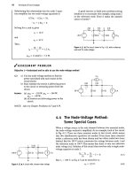
17.1 Use the defining integral to find the Fourier
17.2
The Fourier transform of f(t) is given by
transform of the following functions:
_,, .
6
F(o))
=
0, -oo
<

a)
<
-3;
a)
f(t)
=
-A, -r/2 < t
< 0;
F((o) =
^
_
3
<
<,
<
_
2;
f{t)
« A
0<f<r/2;
F(C)
=
1,
-2<O,<2;
fit)
= 0
elsewhere.
F(ft))
m
4>

2
<
co
< 3;
b)
fit)
= 0,
t
< 0;
F{a)) = 0i 3
<
w
<
oo.
/
.
/2A\f.
O>T\
Answer:
(a) -/I
—
II 1
-
cos—
I;
1
1
(b)
—«.
Answer: f(?)

=
—(4 sin 3t
-
3 sin 2f).
(rt
+
JO))"
TTt
NOTE: Also try Chapter Problems 17.1 and 17.2.
17.3
Using Laplace Transforms
to
Find Fourier Transforms
We can use a table of unilateral, or one-sided, Laplace transform pairs to
find the Fourier transform of functions for which the Fourier integral con-
verges.
The Fourier integral converges when all the poles of F(s) lie in the
left half of the s plane. Note that if F(s) has poles in the right half of the
s plane or along the imaginary axis,/(/) does not satisfy the constraint that
Xoo
1/(01*
exists.
The following rules apply to the use of Laplace transforms to find the
Fourier transforms of such functions.
1.
If /(/) is zero for
t ^
0~, we obtain the Fourier transform of
f(t)
from the Laplace transform of /(f) simply by replacing

5
by
jco.
Thus
*{/(0) «2{/(0W
(
17
-
19
)
17.3 Using Laplace Transforms to Find Fourier Transforms 651
For example, say that
f(0 = 0,
t ^ 0~
fit) = e "
f
cosw
(
/,
0
+
.
Then
*{/(/)}
s + a
jco + a
(s + a)
2
+ (nl
x

=j
lo
(jco + a)
2
+
(x)f)
2.
Because the range of integration on the Fourier integral goes from
— oo
to +oo, the Fourier transform of a negative-time function
exists.
A negative-time function is nonzero for negative values of
time and zero for positive values of time. To find the Fourier trans-
form of such a function, we proceed as follows. First, we reflect the
negative-time function over to the positive-time domain and then
find its one-sided Laplace transform. We obtain the Fourier trans-
form of the original time function by replacing s with -jco.
Therefore, when f(t) = 0 for t > 0
+
,
Hf(*)}
=
-^1/(-01.=-
;w
(17.20)
For example, if
fit) = 0,
(for t > 0
+
);

then
/(/) =
Aosfttf,
(for / < 0").
/(-0 - o.
(for t < 0");
/(-0 = <T'"cosw
(
/, (for t > 0
+
).
Both /(/') and its mirror image are plotted in Fig. 17.5.
The Fourier transform of /(/) is
9{f{t)}
=
W(~0h=
/a
-jco + a
s + a
(s + a) +
COQ
s=-
/w
(-jo + a)
2
+ &Ȥ
Figure 17.5 • The reflection of
a
negative-time
function over to the positive-time domain.

3.
Functions that are nonzero over all time can be resolved into positive-
and negative-time functions. We use Eqs. 17.19 and 17.20 to find the
Fourier transform of the positive- and negative-time functions, respec-
tively.
The Fourier transform of the original function is the sum of the
two transforms. Thus if we let
then
and
A/) =/(0 (for r>0),
/-(/) = /(0 (for/<0),
/(o
=
no
+
/"(o
= ^{/
+
(0},=ya> + ie{/-(-0}.v=-
;w
. (17.21)
An example of using Eq. 17.21 involves finding the Fourier trans-
form of
e
_a
''L
For the original function, the positive- and negative-
time functions are
/
+

(0 = e~
ul
and /"(/) = e'".
Then
2{/
+
(0}
i
S + a
1
s + a
Therefore, from Eq.
17.21,
&{
e
-<to\}
1
s + a
1
+
S= I (it
+
s + a
1
s=—ju)
jo) + a —jo) + a
2a
2
'< 2"
o) + a

If/(0 i
s
even, Eq. 17.21 reduces to
9{f(*)) = %{f(t)}.s=
jt
o + ^{/(01,=-/0,-
If/(/) is odd, then Eq. 17.21 becomes
9{f{t)} = %{f(t)}
s=ia
-
2{/(/)},~/
(17.22)
(17.23)
17.4 Fourier Transforms
in the
Limit
653
/ASSESSMENT PROBLEM
Objective
1—Be
able
to
calculate
the
Fourier transform
of a
function
17.3 Find the Fourier transform
of
each function.

In
each
case,
a
is a positive real constant.
a)
f{t) = 0,
fit)
= e
"'smcoyt,
b)
f(t) = 0,
/(0
=
-te
at
,
c)
f(t) =
te-
(,t
,
/(0
= to",
t
< 0,
t
> 0.
t
> 0,

t
< 0.
t
> 0,
t
s 0.
Answer:
(a)
(b)
OiQ
(c)
(a
+
jco)
2
+ col'
1
(a
-
jco)
2,
-j4aa)
NOTE: Also
try
Chapter Problem 17.5.
17A Fourier Transforms
in the
Limit
As
we

pointed
out in
Section 17.2,
the
Fourier transforms
of
several prac-
tical functions must
be
defined
by a
limit process. We
now
return
to
these
types
of
functions
and
develop their transforms.
{a
1
+ <«/)
2\2'
The Fourier Transform of a Signum Function
We showed that
the
Fourier transform
of a

constant
A is
2TTA8((O)
in
Eq.
17.18.
The next function
of
interest
is the
signum function, defined
as
+
1
for / > 0 and -1 for t <
O.The signum function
is
denoted sgn(0
and
can
be
expressed
in
terms
of
unit-step functions,
or
sgn(0
- u(t) -
u(-t).

(17.24)
Figure 17.6 shows
the
function graphically.
To find
the
Fourier transform
of the
signum function, we first create
a
function that approaches
the
signum function
in the
limit:
sgn(r)
=
lim[e~
€t
u(t)
-
e
et
u(-t)],
e > 0.
£->()
(17.25)
The function inside
the
brackets, plotted

in
Fig. 17.7,
has a
Fourier trans-
form because
the
Fourier integral converges. Because
/(0 is an odd
func-
tion, we
use Eq.
17.23
to
find
its
Fourier transform:
9^(/(0}
1
S
+ €
1
1
s=)to
S
+ €
1
s=—]u>
joo
+ e
—jco

+ e
_ -2jco
a)
2
+ e
2
'
As
e ->
0,
/(0 -»
sgn(0,
and
^{/(0} ~*
2/>.
Therefore,
^{sgn(0}
= —•
(17.26)
sgn(/)
1.0
-1.0
Figure
17.6 •
The signum function.
eM-t)
-1.0
(17
27) Rw* 17.7 A A
function that approaches sgn(r)

as
e approaches zero.
The Fourier Transform of a Unit Step Function
To find the Fourier transform of a unit step function, we use Eqs. 17.18 and
17.27.
We do so by recognizing that the unit-step function can be
expressed as
"(') = - + -sgn(f). (17.28)
Thus,
^2
(
+
H^
s
§
n
(
r
)
=
TT8(O))
+ —.
(17.29)
7*>
The Fourier Transform of a Cosine Function
To find the Fourier transform of cos
o)
()
t,
we return to the inverse-transform

integral of Eq. 17.9 and observe that if
F(<o) =
2TT8(O)
- a>o),
(17.30)
then
l r
/(?) = — /
\2TTS{O)
-
o)
{)
)]e"°'
do).
(17.31)
Using the sifting property of the impulse function, we reduce Eq. (17.31) to
f(t) = e
M>r
. (17.32)
Then, from Eqs. 17.30 and 17.32,
<${e<^} = 2ir8(a)-a)
{)
). (17.33)
We now use Eq. 17.33 to find the Fourier transform of cos
w
()
r,
because
e
hvf +

e
~m\t
cos ay = . (17.34)
Thus,
^{cosa>
0
/} =-(3=(^} + ^{e'
j0
^})
—
[2TT8((O
— wo) +
2TT8((O
+ £%)]
=
TT8((O
— ojo)
+
TT8(O)
+ G>o). (17.35)
17.5
Some
Mathematical Properties
655
The Fourier transform of sin
co
0
t
involves similar manipulation, which
we leave for Problem

17.4.
Table 17.1 presents a summary of the transform
pairs of the important elementary functions.
We now turn to the properties of the Fourier transform that enhance our
ability to describe aperiodic time-domain behavior in terms of frequency-
domain behavior.
TABLE
17.1
Fourier
Transforms
of
Elementary
Functions
Type
impulse
constant
signum
step
positive-time exponential
negative-time exponential
positive- and negative-time exponential
complex exponential
cosine
sine
/(')
8(t)
A
sgn(/)
u(t)
e-

in
u{t)
e
m
u(-t)
e
-«\'\
e/w
COS
0)()1
sin
corf
F(co)
I
2TTA8(CO)
2//oi
7T8((X))
+ 1//(1)
l/(n + /ftj), a > 0
l/(« - /«), a > 0
2a/(a
2
+ or), a > 0
2TT8{(0
— too)
7r[5(o>
+ (0()) + (5((0 -
/V[5(o) + (o
()
)

—
5(a; •
mi)]
~ «,,)]
17.5 Some Mathematical Properties
The first mathematical property we call to your attention is that F(co) is a
complex quantity and can be expressed in either rectangular or polar
form. Thus from the defining integral,
/
00
f{t)e-'
Mt
dt
CXJ
•J
/(/)(cos
cot
- j sin
cot)
dt
L
f(t) cos
cot cit
- j f (t) sin
cot
dt. (17.36)
Now we let
M&) = / f(0
COS cot cit
(17.37)

-X
fi(o)) = -/ /(/) sin mtdt. (17.38)
J—no
Thus,
using the definitions given by Eqs. 17.37 and 17.38 in Eq.
17.36,
we get
F(co) = A(a>) + /£(<«>) = |F(ft>)|e^
M
. (17.39)