Electric Circuits, 9th Edition P75 pdf

If we let C = adj A
•
A and use the technique illustrated in Section A.7,
we find the elements of C to be
Therefore
C =
=
cu
C\2
^13
^21
c
22
c
23
C31
C32
^33
~-8
0
0
Jet A
= 9 -
= 18
= 27
21 +4=-
8,
- 14 - 4 = 0,
- 7 - 20 = 0,
= -16 + 24 - 8 = 0,
= -32 + 16 + 8 = -8,

= -48 + 8 + 40 = 0,
= 5 -
= 10
= 15
0
-8
0
•u.
9 + 4 = 0,
-6-4 = 0,
- 3 - 20 = -8.
0"
0
-8_
= -8
"l 0
0 1
_0 0
0
0
1
A square matrix A has an inverse, denoted as A ',
if
A
-1
A = AA
_1
= U.
(A.50)
Equation A.50 tells us that a matrix either premultiplied or postmultiplied

by its inverse generates the identity matrix U. For the inverse matrix to
exist, it is necessary that the determinant of A not equal zero. Only square
matrices have inverses, and the inverse is also square.
A formula for finding the inverse of a matrix is
A-
!
=
detA
(A.51)
The formula in Eq.
A.51
becomes very cumbersome if A is of an order
larger than 3 by
3.
2
Today the digital computer eliminates the drudgery
of having to find the inverse of a matrix in numerical applications of
matrix algebra.
It follows from
Eq.
A.51
that the inverse of the matrix A in the previ-
ous example is
-1 _
A
-1
= -1/8
9
16
5

-7
8
-3
-4
8
~4_
-1.125 0.875
2 -1
-0.625 0.375
-1A
_
1 i
You should verify that A
l
A = AA = U.
0.5
-1
0.5
2
You can learn alternative methods for finding the inverse in any introductory text on
matrix theory. See, for example, Franz E. Hohn, Elementary Matrix Algebra (New York:
Macmillan, 1973).
A.9 Partitioned Matrices
It is often convenient in matrix manipulations to partition a given matrix
into
submatrices.
The original algebraic operations are then carried out in
terms of the submatrices. In partitioning a matrix, the placement of the
partitions is completely arbitrary, with the one restriction that a partition
must dissect the entire matrix. In selecting the partitions, it is also neces-

sary to make sure the submatrices are conformable to the mathematical
operations in which they are involved.
For example, consider using submatrices to find the product
C = AB, where
A =
1
5
1
0
0
2
4
0
1
2
3
3
2
-1
1
4
2
-3
0
-2
5
1
1
1
0

and
B
2
0
-1
3
0
Assume that we decide to partition B into two submatrices, B
n
and
B
2
j;
thus
B
B21
Now since B has been partitioned into a two-row column
matrix,
A must be
partitioned into at least a two-column matrix; otherwise the multiplication
cannot be performed.
The
location of the vertical partitions of the A matrix
will depend on the definitions of B
n
and B
2
i. For example,
if
B,

and B
21
then An must contain three columns, and A
12
must contain two columns.
Thus the partitioning shown in Eq. A.52 would be acceptable for execut-
ing the product AB:
C =
1 2
5 4
-1 0
0 1
0 2
3
3
2
-1
1
4 5~
2 1
3 1
0 1
2 0_
2~
0
-1
3
0_
(A.52)
If, on the other hand, we partition the B matrix so that

B
n
-
2
.0.
and B?i =
-1
3
0
then An must contain two columns, and A
12
must contain three columns.
In this case the partitioning shown in Eq. A.53 would be acceptable in exe-
cuting the product C = AB:
C =
1
5
1
0
0
2
4
0
1
2
3
3
2
-1
1

4
2
-3
0
-2
5~
1
1
1
0_
2
0
-1
3
0
(A.53)
For purposes of discussion, we will focus on the partitioning given in
Eq. A.52 and leave you to verify that the partitioning in Eq. A.53 leads to
the same result.
From Eq. A.52 we can write
C = [A
n
A
12
]
B„
= A
n
B
n

+ A
12
B
21-
(A. 54)
It follows from Eqs. A.52 and A.54 that
A,,B
ll*»1l
1 2
5 4
-1 0
0 1
0 2
3~
3
2
1
1
2~
0
_-!_
=
~-l"
7
-4
1
_-!_
A12B21 -
4 5~
2 1

-3 1
0 1
_~2 0_
"3"
.0.
=
~ 12"
6
-9
0
_-6_
and
11
13
-13
1
-7
The A matrix could also be partitioned horizontally once the vertical
partitioning is made consistent with the multiplication operation. In this
simple problem, the horizontal partitions can be made at the discretion of
the analyst. Therefore C could also be evaluated using the partitioning
shown in Eq.A.55:
1
5
1
0
0
?
4
0

1
2
3
3
2
-1
1
5
1
1
1
0_
2~
0
-1
3
0_
(A.55)
From Eq. A.55 it follows that
An
A
21
A
12
A,?
B,i
B„
LC
21
(A.56)

where
You should verify that
Cj!
- A
u
B
n
+ A
I2
B
2
|,
C
2
i = A
21
B
11
+
A22B21.
C„ =
1 2 3
5 4 3
+
4 5
2 1
-1
7
+
12

6
=
11
13
c„ =
-1 0
0 1
0 2
2~
1
1_
2~
0
_-!_
+
"-3
0
_-2
r
1
0_
"3*
.0.
-4
1
-1
+
-9
0
-6

=
-13
1
-7
and
C =
11
13
-13
1
-7
We note in passing that the partitioning in Eqs. A.52 and A.55 is
conformable with respect to addition.
720
The
Solution of Linear Simultaneous Equations
A.10 Applications
The following examples demonstrate some applications of matrix algebra
in circuit analysis.
Example A.l
Use the matrix method to solve for the node volt-
ages V\ and v
2
in Eqs. 4.5 and 4.6.
Solution
The first step is to rewrite Eqs. 4.5 and 4.6 in matrix
notation. Collecting the coefficients of «, and v
2
and at the same time shifting the constant terms to
the right-hand side of the equations gives us

1.7«! - 0.5¾ = 10,
(A.57)
-0.5«] + 0.6«
2
= 2.
It follows that in matrix notation, Eq. A.57 becomes
1.7
-0.5
•0.5
0.6
10
2
or
where
AV = I,
(A.58)
(A.59)
A
A.
—
V =
I =
1.7
().5
V
'10"
. 2.
•
•
-0.5"

0.6.
To find the elements of the V matrix, we pre-
multiply both sides of Eq. A.59 by the inverse of
A; thus
or
A
_1
AV = A
_1
I.
Equation A.60 reduces to
UV = A
"T,
V = A
"I.
(A.60)
(A.61)
(A.62)
It follows from Eq. A.62 that the solutions for
V\ and v
2
are obtained by solving for the matrix
product A
-1
1.
To find the inverse of A, we first find the
cofactors of A. Thus
A
H
= (-1)

2
(0.6) = 0.6,
A12 = (-l)
3
(-0.5) = 0.5,
A
2
i = ("l)
3
(-0.5) = 0.5,
A22 = (-l)
4
(l-7) = 1.7.
The matrix of cofactors is
(A.63)
B
0.6
0.5
and the adjoint of A is
adj A = B
7
=
The determinant of A is
0.5
1.7
0.6
L0.5
0.5
1.7
(A.64)

(A.65)
detA
1.7
-0.5
-0.5
0.6
(1.7)(0.6) - (0.25) = 0.77.
(A.66)
From Eqs. A.65 and A.66, we can write the inverse
of the coefficient matrix, that is,
(A.67)
A"
1
1
0.77
0.6
.0.5
0.5
1.7
Now the product A
-1
1 is found:
A-I = ^
77
0.6 0.5"
.0.5 1.7.
loor 7"
77 U.4 _ "
"10
. 2

" 9.09"
.10.91.
It follows directly that
V
v
2
-
' 9.09'
.1
3.91
'
(A.68)
(A.69)
or vj = 9.09 V and v
2
= 10.91 V.
A.10 Applications
721
Example A.2
Use the matrix method to find the three mesh cur-
rents in the circuit in Fig. 4.24.
Solution
The mesh-current equations that describe the cir-
cuit in Fig. 4.24 are given in Eq. 4.34. The constraint
equation imposed by the current-controlled voltage
source is given in Eq.
4.35.
When Eq. 4.35 is substi-
tuted into Eq. 4.34, the following set of
equations evolves:

25/,-
- 5/
2
- 20/
3
= 50,
-5/,
- 4z
2
+ 9/
3
= 0.
In matrix notation, Eqs. A.70 reduce to
AI = V,
where
A =
(A.70)
(A.71)
and
25 -5
-5 10
-5 -4
'*]
h
h_
1
V =
r
50"
0

0
-20
-4
9
.
It follows from Eq.
A.71
that the solution for I is
I = A
1
V. (A.72)
We find the inverse of A by using the relationship
A
-
' =
_ adjA
detA
(A.73)
To find the adjoint of A, we first calculate the cofac-
tors of
A.
Thus
An = (-1)
2
(90 - 16) = 74,
A12 = (-l)
3
(-45 - 20) = 65,
A13 = (-1)^(20 + 50) = 70,
A21 = (-l)

3
(-45 - 80) = 125,
A22 =
A 23 =
A
3
1 = I
A
32
=
<
A33 = (
;-l)
4
(225 - 100) = 125,
;-l)
5
(-100 - 25) = 125,
;-l)
4
(20 + 200) = 220,
-1)
5
(-100 - 100) = 200,
-1)
6
(25() - 25) = 225.
The cofactor matrix is
B
74 65 70

125 125 125
220 200 225
(A.74)
from which we can write the adjoint of A:
adj A = B
r

74
65
_70
The determinant of A is
detA =
25 -5 -20
-5 10 -4
-5 -4 9
125
125
125
220
200
225
(A.75)
= 25(90 -16) + 5(-45 - 80) - 5(20 + 200) = 125.
It follows from Eq. A.73 that
-1 _
1
125
74 125 220
65 125 200
70 125 225

(A.76)
The solution for I is
1
125
74 125
65 125
70 125
220
200
225
50
0
0
=
29.60
26.00
28.00
. (A.77)
The mesh currents follow directly from
Eq. A.77.
Thus
(A.78)
or /j = 29.6 A, i
2
= 26 A, and /
3
= 28 A.
Example A.3 illustrates the application of the
matrix method when the elements of the matrix are
complex numbers.

h
h
_*3_
=
"29.6"
26.0
_28.0_
722 The Solution of Linear Simultaneous Equations
Example A.3
Use the matrix method to find the phasor mesh cur-
rents I, and I
2
in the circuit in Fig. 9.37.
Solution
Summing the voltages around mesh 1 generates
the equation
(1 + /2)1, + (12 -
/16)(1,
- I
2
) = 150/0". (A.79)
Summing the voltages around mesh 2 produces
the equation
(12 - /16)(I
2
- Ii) + (1+ /3)I
2
+ 39I
V
= 0.(A.80)

The current controlling the dependent voltage
source is
I, = (Ii - I
2
)-
(A.81)
After substituting Eq. A.81 into Eq. A.80, the
equations are put into a matrix format by first collect-
ing,
in each equation, the coefficients of I, and I
2
: thus
(13 -
/14)1,
- (12 - /16)I
2
= 150/0°,
(27 +
/16)1,
- (26 + /13)¾ = 0.
Now, using matrix notation, Eq. A.82 is written
(A.82)
where
A =
I
AI = V,
13 - /14 -(12 - /16)
[27 + /16 -(26 + /13)
(A.83)
and V

150/0
0
It follows from Eq. A.83 that
I = A V. (A.84)
The inverse of the coefficient matrix A is found
using Eq.
A.73.
In this case, the cofactors of A are
^
n
= (-l)
2
(-26-/13) =
-26-/13,
A
12
= (-l)
3
(27 + /16) = -27-/16,
A
2
i = (-1)
3
(-12 + /16) = 12 - /16,
A
22
= (-1)
4
(13 - /14) = 13 - /14.
The cofactor matrix B is

B =
The adjoint of A is
adj A = B
7
=
The determinant of A is
detA =
(-26 - /13) (-27 - /16)
(12-/16) (13-/14)
(-26 - /13) (12 - /16)
L(-27-/16) (13-/14)J
(A.85)
(A.86)
(13 - /14)
(27 + /16)
(12 - /16)
(26 + /13)
= -(13 - /14)(26 + /13) + (12 - /16)(27 + /16)
= 60 - /45. (A.87)
The inverse of the coefficient matrix is
A~
!
=
(-26-/13) (12-/16)
L(-27 -/16) (13 -/14)J
(60 - /45)
Equation A.88 can be simplified to
(A.88)
60 + /45
5625

(-26 - /13) (12 - /16)
(-27 - /16) (13 - /14)
1
375
-65 - /130 96 - /28
-60 - /145 94 - /17
(A.89)
Substituting Eq. A.89 into A.84 gives us
1
375
(-65 - /130) (96 - /28)
(-60 - /145) (94 - /17)
150/0
C
0
(-26 - /52)
(-24 - /58)
It follows from Eq. A.90 that
I, = (-26 - /52) = 58.14/-116.57° A,
h = (-24 - /58) = 62.77/-122.48° A.
(A.90)
(A.91)
In the first three
examples,
the matrix elements have been numbers—real
numbers in Examples A.l and A.2, and complex numbers in Example
A.3.
It
is also possible for the elements to be functions. Example A.4 illustrates the
use of matrix algebra in a circuit problem where the elements in the coeffi-

cient matrix are functions.
A.10 Applications 723
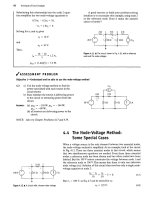
Example A.4
Use the matrix method to derive expressions for
the node voltages
V
x
and
V
2
in the circuit in Fig. A.
1.
Solution
Summing the currents away from nodes 1 and 2
generates the following set of equations:
R
+
V
x
sC
+ (K, -
V
2
)sC
= 0,
f + (½ ~ VfisC +
(V
2
-
V

g
)sC
= 0.
(A.92)
Letting G = \/R and collecting the coefficients of
V]
and
V
2
gives us
(G + 2sC)Vi -
sCV
2
= GVp
-sCVi + (G +
2sC)V
2
=
sCV
R
.
Writing Eq. A.93 in matrix notation yields
AV = I,
where
(A.93)
(A.94)
G + 2sC
-sC
v
2

.
, and
—5
C
G + 2sC_
I -
_sCV
i
V =
It follows from Eq. A.94 that
V - A'l. (A.95)
As before, we find the inverse of the coefficient
matrix by first finding the adjoint of A and the
determinant of A. The cofactors of A are
A
n
= (-1)
2
[G + 2sC] = G + 2sC,
A
12
= (-l)\sC) = sC,
A
2
i = {-l)\sC) - sC,
A22 = (~1)
4
[G + 2sC] = G + 2sC.
The cofactor matrix is
G + 2sC

B -
sC
sC
G + 2sC
(A.96)
and therefore the adjoint of the coefficient matrix is
I
G + 2sC sC
sC G + 2sC
adj A = B
7
(A.97)
Figure A.l • The circuit for Example A.4.
The determinant of A is
G + 2sC sC
detA = „ _ „ _
sC G + 2sC
= G
2
+ 4sCG + 3.v
2
C
2
.
(A.98)
The inverse of the coefficient matrix is
A~
l
=
G + 2sC sC

sC G + 2sC
(G
2
+ AsCG + 3.v
2
C
2
)
(A.99)
It follows from Eq. A.95 that
G + 2sC sC
sC G + 2sC
sCV
a
{G
z
+ AsCG + 3s
l
C
l
)
(A.100)
Carrying out the matrix multiplication called for in
Eq.A.100 gives
V
2
J
(G
2
+ 4.vCG + 3.v

2
C
2
)
(G
2
+ 2sCG +
s
2
C
2
)V
g
(2sCG +
2s*C
2
)V
n
(A.101)
Now the expressions for V\ and V
2
can be written
directly from Eq. A.
101;
thus
(G
2
+ 2sCG +
s
2

C
2
)V
K
V\ = ,w> . . ^ . „ ^ »
(
A
-
102
)
(G
2
+ 4sCG + 3s
2
C
2
) '
and
2^
v>
=
2(sCG + s
l
C
z
)V<,
(G
2
+ 4sCG + 3s
2

C
2
)
(A.103)
724 The Solution of Linear Simultaneous Equations
In our final example, we illustrate how matrix algebra can be used to
analyze the cascade connection of two two-port circuits.
Example A.5
Show by means of matrix algebra how the input
variables
V
x
and Iy can be described as functions of
the output variables V
2
and I
2
in the cascade con-
nection shown in Fig. 18.10.
Solution
We begin by expressing, in matrix notation, the
relationship between the input and output variables
of each two-port
circuit.
Thus
(A.104)
and
(A.105)
Vi
/J

v\
/',
«il
.«21
r«u
ki
-«12
~«22-
-«12]
~«22 J
v
2
L/2
\v
2
lh
Now the cascade connection imposes the constraints
V'
2
= V\ and
1'
2
= -J\. (A.106)
These constraint relationships are substituted into
Eq.
A.104.
Thus
«h
«21
«ii

«21
-«12
-«22
«12
«22-
-I'u
L/'I
(A.107)
The relationship between the input variables (V
h
/j)
and the output variables (V
2
, J
2
) is obtained by
substituting
Eq.
A.105
into
Eq.
A.107.
The result is
«11
«23
«12
«22
«11
L«
2

'i
-«12
"«22J
v
2
L/2
(A.108)
After multiplying the coefficient matrices, we have
V
2
Vi
LA
(«il«ll + «12«2l)
(«21«11 + «22«2l)
-
(«11«']2 + «12«22)
-(«21«12 + «22«22)J L/2
(A.109)
Note that Eq.A.109 corresponds to writing
Eqs.
18.72
and
18.73
in matrix form.
Appendix
Q Complex Numbers
Complex numbers were invented to permit the extraction of the square roots
of negative numbers. Complex numbers simplify the solution of problems
that would otherwise be very difficult. The equation x
2

+ 8x + 41 = 0,
for example, has no solution in a number system that excludes complex
numbers. These numbers, and the ability to manipulate them algebraically,
are extremely useful in circuit analysis.
B.l Notation
There are two ways to designate a complex number: with the cartesian, or
rectangular, form or with the polar, or trigonometric, form. In the
rectangular form, a complex number is written in terms of its real and
imaginary components; hence
n = a + jb, (B.l)
where a is the real component, b is the imaginary component, and ; is by
definition V-l.
1
In the polar form, a complex number is written in terms of its magni-
tude (or modulus) and angle (or argument); hence
n = ce
je
(B.2)
where c is the magnitude, 6 is the angle, e is the base of the natural loga-
rithm, and, as before, j = V-T. In the literature, the symbol /6° is fre-
quently used in place of e
jB
\ that is, the polar form is written
n = c/6°. (B.3)
Although Eq. B.3 is more convenient in printing text material, Eq. B.2 is of
primary importance in mathematical operations because the rules for
manipulating an exponential quantity are well known. For example, because
(
7
7> =

y
*»,then(e^)" =
e
jn6
\
because v"
v
= l/y\ then e'
10
= l/e^;and
so forth.
Because there are two ways of expressing the same complex number,
we need to relate one form to the other. The transition from the polar to
the rectangular form makes use of Euler's identity:
e.
±ie
= cos 6 ± /sin 6. (B.4)
1
You may be more familiar with the notation i = y/^. In electrical engineering, / is used
as the svmbol for current, and hence in electrical engineering literature,/ is used to denote