Electric Circuits, 9th Edition P76 ppt

726 Complex Numbers
A complex number in polar form can be put in rectangular form by writing
ce
je
= c(cos0 + /sin 0)
= c cos 0 + jc sin 0)
= a + jb.
(B.5)
The transition from rectangular to polar form makes use of the geom-
etry of the right triangle, namely,
a + jb = Va
2
+ b
2
)e
je
= ce
j0
(B.6)
where
tan0 = b/a.
(B.7)
It is not obvious from Eq. B.7 in which quadrant the angle 0 lies. The ambi-
guity can be resolved by a graphical representation of the complex number.
b
0
s^
H
J?\
C
a

Figure B.l • The graphical representation of a + jb
when a and b are both positive.
I
l
5 36.87° 5
4
4+/3 = 5/36.87°
(a)
143.13° '
\
3
1
1 1 1
IX
-4
J/l
1
1
i
i i ;
l.
-4 + /3 = 5,/143.13°
(b)
i
i 1
il
U
-4,
-3
5 216.87°

-4-/3 = 5/216,87
0
(c)
i_L
0
1
1 1 1 1 I
-3
i_
~l 1
ZyS
—
5
1 1 1
4
s
323.
1,
13°
4-/3
= 5/323.13°
(d)
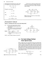
Figure B.2 A The graphical representation of four
complex numbers.
B.2 The Graphical Representation
of a Complex Number
A complex number is represented graphically on a complex-number
plane, which uses the horizontal axis for plotting the real component and
the vertical axis for plotting the imaginary component. The angle of the
complex number is measured counterclockwise from the positive real axis.

The graphical plot of the complex number n = a + jb = c /0°, if we
assume that a and b are both positive,is shown in Fig. B.l.
This plot makes very clear the relationship between the rectangular and
polar forms. Any point in the complex-number plane is uniquely defined by
giving either its distance from each axis (that is, a and b) or its radial dis-
tance from the origin (c) and the angle of the radial measurement 0.
It follows from Fig. B.l that 0 is in the first quadrant when a and b are
both positive, in the second quadrant when a is negative and b is positive,
in the third quadrant when a and b are both negative, and in the fourth
quadrant when a is positive and b is negative. These observations are
illustrated in Fig. B.2, where we have plotted 4 + /3, -4 + /3, -4 - /3,
and 4-/3.
Note that we can also specify 0 as a clockwise angle from the positive
real axis. Thus in Fig. B.2(c) we could also designate —4 - /3 as
5/-143.13°. In Fig. B.2(d) we observe that 5/323.13° = 5/-36.87°. It is
customary to express 0 in terms of negative values when 0 lies in the third
or fourth quadrant.
The graphical interpretation of a complex number also shows the
relationship between a complex number and its conjugate. The conjugate
of a complex number is formed by reversing the sign of its imaginary
component. Thus the conjugate of a + jb is a - jb, and the conjugate of
—a + jb is — a - jb. When we write a complex number in polar form, we
form its conjugate simply by reversing the sign of the angle 0. Therefore
the conjugate of c/0° is c/-0°. The conjugate of a complex number is
B.3 Arithmetic Operations 727
designated with an asterisk. In other words, n* is understood to be the /j, = -a+jb-c
&•>
conjugate of n. Figure B.3 shows two complex numbers and their conju-
gates plotted on the complex-number plane.
Note that conjugation simply reflects the complex numbers about the

real axis.
/j
= — a+ib—v #->
^. " d-
~
a
^^
-b-
112 —
—u-jb=c -H2
n
^f
^¾^
«] =
-
(i-
«+
~jb =
b = c 0,
1
a
c -0
{
B.3 Arithmetic Operations
Addition (Subtraction)
To add or subtract complex numbers, we must express the numbers in rec-
tangular form. Addition involves adding the real parts of the complex
numbers to form the real part of the sum, and the imaginary parts to form
the imaginary part of the sum. Thus, if we are given
Figure B.3 A The complex numbers n

x
and n
2
amd their
conjugates n\ and «3.
and
then
«! = 8 + /16
«2 = 12 - /3,
n
{
+ n
2
= (8 + 12) + /(16 - 3) = 20 + /13.
Subtraction follows the same
rule.
Thus
n
2
- «j = (12 -8)+ /(-3 - 16) = 4 - /19.
If the numbers to be added or subtracted are given in polar form, they are
first converted to rectangular form. For example, if
«i = 10/53.13°
and
then
and
n
2
= 5/-135°,
m + n

2
= 6 + /8 - 3.535 - /3.535
= (6 - 3.535) + /(8 - 3.535)
= 2.465 + /4.465 = 5.10/61.10°,
/11 - n
2
= 6 + /8- (-3.535 - /3.535)
= 9.535 + /11.535
= 14.966 /50.42°.
Multiplication (Division)
Multiplication or division of complex numbers can be carried out with the
numbers written in either rectangular or polar form. However, in most
cases,
the polar form is more convenient. As an example, let's find the
product n
x
n
2
when /^ = 8 + /10 and n
2
= 5 - /4. Using the rectangular
form, we have
n
x
n
2
= (8 + /10)(5 - /4) = 40 - /32 + /50 + 40
= 80 + /18
= 82/12.68°.
If we use the polar form, the multiplication n.\n

2
becomes
n
1
n
2
= (12.81 /51.34° )(6.40 /-38.66° )
= 82/12.68°
= 80 + /18.
The first step in dividing two complex numbers in rectangular form is to
multiply the numerator and denominator by the conjugate of the denomi-
nator. This reduces the denominator to a real number. We then divide the
real number into the new numerator. As an example, let's find the value of
n\/n
2
, where rt\ = 6 + /3 and n
2
= 3 -
/1.
We have
«1
n
2
6 + /3
3 - /1
(6 +
(3-
18 + /6 + /9 -
9 + 1
15 + /15

10
= 2.12 /45°
/3)(3 +
/1)(3 +
-3
= 1.5 + /1.5
/1)
/1)
In polar form, the division of n
x
by n
2
is
n
{
6.71 /26.57°
n
2
3.16/-18.43°
= 1.5 + /1.5.
2.12 /45'
B.4 Useful Identities
In working with complex numbers and quantities, the following identities
are very useful:
± /
2
= + 1, (B.8)
(-/)(/)
= U (B.9)
/ = ^7, (B.10)

ff
*/»/2 =
±
/. (B.i2)
Given that n = a + jb = c/0°, it follows that
nn = a
2
+ b
z
= <r, (B.13)
« + n = 2«, (B.14)
n - n* = jib, (B.15)
«/w* =
1/20°.
(B.16)
B.5 The Integer Power
of a Complex Number
To raise a complex number to an integer power k, it is easier to first write
the complex number in polar form. Thus
n
k
= (a + jb)
k
= (cei°)
k
= c
k
e
jk0
= c

k
(coskd + j sinkO).
For example,
(2e
/12
°)
5
= 2V
6()
° = 32e
mr
= 16
+)27.71,
and
(3 + /4)
4
=
(5e^
y
)
4
= 5V
m52
°
= 625^
212,52
°
= -527 - /336.
B.6 The Roots of a Complex Number
To find the /cth root of a complex number, we must recognize that we are

solving the equation
x
k
-ce'
6
= 0, (B.17)
which is an equation of the kth degree and therefore has k roots.
To find the k roots, we first note that
ce
je
= ce
mi*)
= ce
m-w
=

>
(B 18)
It follows from Eqs.
B.17 and B.18
that
Xj
=
(ce'°y
/k
= c
yk
eW\
X
2

=
[
ce
W+2iryil/k
=
c
l/k
e
j{fi+2v)/k^
X$
=
[ce'
i0+47T)
}
]/k
=
c
Vk
e
J(0+47r)/k^
We continue
the
process outlined
by Eqs. B.19, B.20, and B.21
until
the
roots start repeating. This will happen when
the
multiple
of

n
is
equal
to
2k. For
example, let's find
the
four roots
of
81tf
y6{)
°. We have
Xt
=
8lVV6°/4
=
3e'
ls
°,
X2
= 81^/^+360)/4
=
^/1(^
x
3
=
8W
m+m
V
4

=
3e'
195
'\
x
=
g
l
l/4
e
/(6()+ t«H0)/4
=
2e
j2
^'\
Xj
=
81
l/4^(60
+
1440)/4
=
3t
,/375^
=
3^
Here,
x$
is the
same

as
X\,
so the
roots have started
to
repeat. Therefore
we
know
the
four roots
of
81*?
;
are the
values given
by X\,
X
2
, X
3
,
and
X4.
It
is
worth noting that
the
roots
of a
complex number

lie on a
circle
in
the complex-number plane.
The
radius
of the
circle
is
c
!///<
.
The
roots
are
uniformly distributed around
the
circle,
the
angle between adjacent roots
being equal
to
lir/k radians,
or
360/k
degrees.
The four roots
of
81
e

'
6(r
are
shown plotted
in
Fig.
B.4.
3.
105°
/
/
1
1
1• 1 1
3
195°^
"s.
N
_
\
\
fc3
15°
1
i 1 1
1
-
I
/
~

3.
285°
Figure
B.4
•
The
four roots
of
%\e
m
".
(B.19)
(B.20)
(B.21)
Appendix
_ More on Magnetically
{ Coupled Coils and Ideal
Transformers
C.l Equivalent Circuits for Magnetically
Coupled Coils
At times, it is convenient to model magnetically coupled coils with an
equivalent circuit that does not involve magnetic coupling. Consider the
two magnetically coupled coils shown in Fig. C.l. The resistances Ri and
R
2
represent the winding resistance of each
coil.
The goal is to replace the
magnetically coupled coils inside the shaded area with a set of inductors
that are not magnetically coupled. Before deriving the equivalent circuits,

we must point out an important restriction: The voltage between terminals
b and d must be zero. In other words, if terminals b and d can be shorted
together without disturbing the voltages and currents in the original cir-
cuit, the equivalent circuits derived in the material that follows can be
used to model the coils. This restriction is imposed because, while the
equivalent circuits we develop both have four terminals, two of those four
terminals are shorted together. Thus, the same requirement is placed on
the original circuits.
We begin developing the circuit models by writing the two equations
that relate the terminal voltages i?i and v
2
to the terminal currents i
x
and
i
2
. For the given references and polarity dots,
di\ diz
i-h
U-r + M~r
dt dt
(C.l)
and
Vi
du dh
dt dt
(C.2)
«1
+-
'l

a
+
"i
* L*
Ll
)
M
«1
••2 V
2
Figure C.l • The circuit used to develop an equivalent
circuit for magnetically coupled coils.
The T-Equivalent Circuit
To arrive at an equivalent circuit for these two magnetically coupled coils,
we seek an arrangement of inductors that can be described by a set of
equations equivalent to Eqs. C.l and C.2. The key to finding the arrange-
ment is to regard Eqs. C.l and C.2 as mesh-current equations with i
y
and i
2
as the mesh variables. Then we need one mesh with a total inductance of
L\
H and a second mesh with a total inductance of L
2
H. Furthermore, the
two meshes must have a common inductance of M H. The T-arrangement
of coils shown in Fig. C.2 satisfies these requirements.
Figure C.2 • The T-equivalent circuit for the magneti-
cally coupled coils of Fig. C.l.
731

732 More on Magnetically Coupled Coils and Ideal Transformers
You should verify that the equations relating v
Y
and v
2
to /, and i
2
reduce to Eqs. C.l and
C.2.
Note the absence of magnetic coupling between
the inductors and the zero voltage between b and d.
The ^-Equivalent Circuit
We can derive a 7r-equivalent circuit for the magnetically coupled coils
shown in Fig. C.l.This derivation is based on solving Eqs. C.l and C.2 for
the derivatives dijdt and di^jdt and then regarding the resulting expres-
sions as a pair of node-voltage equations. Using Cramer's method for solv-
ing simultaneous equations, we obtain expressions for di\jdt and di
2
/dt:
di\
dt
V\
v
2
u
M
M
L
2
M

L
2
LiL
1^2
M
Vl
M
L
X
L
2
- M
•v
2
;
(C.3)
di
2
dt
M
v
2
•M
UU - M
2
UL
<\^2
1^2
w
Vi +

Li
L,L>,
- M
l
jVl
(C.4)
Now we solve for /, and i
2
by multiplying both sides of Eqs. C.3 and C.4 by
dt and then integrating:
k = *i(0) +
L
X
L
2
- M
2
J{)
V
{
dT
M
L
X
L
2
-
M
l
h

v
2
dr (C.5)
and
'
2
(0)
UU
x / v\dr + r /
M
2
J
{)
L
X
L
2
-M
2
k
v
2
dT.
(C.6)
If we regard v
x
and v
2
as node voltages, Eqs. C.5 and C.6 describe a circuit
of the form shown in Fig. C.3.

All that remains to be done in deriving the 7r-equivalent circuit is to
find L
A
, L
B
, and L
c
as functions of L
h
L
2
, and M. We easily do so by writ-
ing the equations for /
t
and i
2
in Fig. C.3 and then comparing them with
Eqs.
C.5 and
C.6.
Thus
Figure C.3 • The circuit used to derive the 7r-equivalent circuit for
magnetically coupled coils.
C.l Equivalent Circuits for Magnetically Coupled Coils 733
1 f 1 /*'
ii = /j(0) + — / Vidr + — I («! - v
2
)dr
LA
JO

L
B
JO
and
1 /"' 1 /'
*
2
= «2(0) + -^- v
2
dT + — I (v
2
- v
x
)dr
I-C
./0 L3 JO
=
«'
2
(0)
+ 7" / M* +(7- + 7-]
Then
M
L
B
L^ - M
2'
(C.9)
L
A

L
2
-M
L
X
L
2
-
M
2
'
(CIO)
L
c
Li
/V/
LiL
1^2
Mr
(til)
When we incorporate Eqs. C.9-C.11 into the circuit shown in Fig. C.3, the
^-equivalent circuit for the magnetically coupled coils shown in Fig. C.l is
as shown in Fig. C.4.
Note that the initial values of
iy
and i
2
are explicit in the ^-equivalent
circuit but implicit in the T-equivalent circuit. We are focusing on the sinu-
soidal steady-state behavior of circuits containing mutual inductance, so

we can assume that the initial values of ij and i
2
are zero. We can thus
eliminate the current sources in the ^-equivalent circuit, and the circuit
shown in Fig. C.4 simplifies to the one shown in Fig. C.5.
The mutual inductance carries its own algebraic sign in the T- and
^-equivalent circuits. In other words, if the magnetic polarity of the cou-
pled coils is reversed from that given in Fig. C.l, the algebraic sign of M
Figure C.4 A
The
7r-equivalent circuit for the magnetically coupled coils of
Fig.
C.l. Figure C.5 •
The
^-equivalent circuit used for
sinusoidal steady-state analysis.
734 More on Magnetically Coupled Coils and Ideal Transformers
reverses. A reversal in magnetic polarity requires moving one polarity dot
without changing the reference polarities of the terminal currents and
voltages.
Example C.l illustrates the application of theT-equivalent circuit.
Example C.l
a) Use the T-equivalent circuit for the magnetically
coupled coils shown in Fig. C.6 to find the phasor
currents I| and I
2
. The source frequency is
400 rad/s.
b) Repeat (a), but with the polarity dot on the sec-
ondary winding moved to the lower terminal.

Solution
a) For the polarity dots shown in Fig. C.6, M carries
a value of +3 H in the T-equivalent circuit.
Therefore the three inductances in the equiva-
lent circuit are
L
{
- M = 9 - 3 = 6 H;
L
2
- M = 4 - 3 =
1
H;
M = 3 H.
Figure C.7 shows the T-equivalent circuit, and
Fig. C.8 shows the frequency-domain equivalent
circuit at a frequency of 400 rad/s.
Figure C.9 shows the frequency-domain
circuit for the original system.
Here the magnetically coupled coils are
modeled by the circuit shown in Fig.
C.8.
To find
the phasor currents I] and I
2
, we first find the
node voltage across the 1200 O inductive reac-
tance. If we use the lower node as the reference,
the single node-voltage equation is
300

+
900 - /2100
= 0.
700 + y'2500 /1200
Solving for V yields
V = 136 - /8 = 136.24/-3.37° V(rms).
Then
300 -(136- /8)
700 + /2500
63.25 /-71.57° mA (rms)
500
a
/loo
a
_TVYY>_
II
300/0
Q
V
a
200
a /1200 a
4.
o I •
loo
a
800
a
A/W
6H

1 H
|3H
Figure C.7 A The T-equivalent circuit for the magnetically
coupled coils in Example C.l.
/2400 /400
:/1200
Figure C.8 • The frequency-domain model of the equivalent
circuit at 400 rad/s.
500
a
/
loo
a
200
a
/2400
a
/400
a
100
a
6
3()0,()°
V
/I200a
Figure C.9 A The circuit of Fig. C.6, with the magnetically
coupled coils replaced by their T-equivalent circuit.
and
I, =
136 - /8

900 - /2100
59.63 /63.43° mA (rms).
Vi /3600 a
b) When the polarity dot is moved to the lower ter-
minal of the secondary coil, M carries a value of
-3 H in the T-equivalent circuit. Before carrying
out the solution with the new T-equivalent cir-
cuit, we note that reversing the algebraic sign of
M has no effect on the solution for Ij and shifts
I
2
by 180°.Therefore we anticipate that
/2500 a
Figure C.6 A The frequency-domain equivalent circuit for Example C.l.
and
Ij = 63.25/-71.57° mA (rms)
I
2
= 59.63 /-116.57° mA (rms).
We now proceed to find these solutions
by using the new T-equivalent circuit. With
M = -3 H, the three inductances in the equiv-
alent circuit are
Lj - M = 9 - (-3) = 12 H;
L
2
-
M = 4- (-3) = 7H;
M = -3H.
At an operating frequency of 400 rad/s, the

frequency-domain equivalent circuit requires two
inductors and a capacitor, as shown in Fig. CIO.
The resulting frequency-domain circuit for
the original system appears in Fig. C.ll.
As before, we first find the node voltage
across the center branch, which in this case is a
capacitive reactance of — /'1200 H. If we use the
lower node as reference, the node-voltage
equation is
V - 300
+ +
700 + /4900 -/1200 900 + /300
Solving for V gives
V = -8 - /56
= 56.57 /-98.13° V (rms).
C.2 The Need for Ideal Transformers in the Equivalent Circuits 735
Then
300 -(-8- /56)
h =
and
700 + /4900
= 63.25 /-71.57° mA (rms)
-8 - /56
900 + /300
= 59.63 /-116.57° mA (rms).
/4800 fl /2800 0
-/1200O
Figure CIO •
The
frequency-domain equivalent circuit for

M = -3 H and
a>
= 400 rad/s.
500
n
/loo
n
200
n
/48ooa /28oon
1000
r^/
3
°
(
M
jc
I
V
-/120012:
800
O
-/25()0
il
Figure C.ll • The frequency-domain equivalent circuit for
Example C.l(b).
C.2 The Need for Ideal Transformers in
the Equivalent Circuits
The inductors in the T- and 77-equivalent circuits of magnetically cou-
pled coils can have negative values. For example, if L\ = 3 mH,

L
2
= 12 mH, and M = 5 mH, the T-equivalent circuit requires an induc-
tor of
—2
mH, and the 7r-equivalent circuit requires an inductor of
-5.5 mH. These negative inductance values are not troublesome when
you are using the equivalent circuits in computations. However, if you
are to build the equivalent circuits with circuit components, the negative
inductors can be bothersome. The reason is that whenever the frequency
of the sinusoidal source changes, you must change the capacitor used to
simulate the negative reactance. For example, at a frequency of
50 krad/s, a -2 mH inductor has an impedance of -/100 fi.This imped-
ance can be modeled with a capacitor having a capacitance of 0.2 /xF. If
the frequency changes to 25 krad/s, the -2 mH inductor impedance
changes to -/50 il. At 25 krad/s, this requires a capacitor with a capaci-
tance of 0.8 /xF. Obviously, in a situation where the frequency is varied