Electric Circuits, 9th Edition P77 ppsx

736 More on Magnetically Coupled Coils and Ideal Transformers
continuously, the use of a capacitor to simulate negative inductance is
practically worthless.
You can circumvent the problem of dealing with negative inductances
by introducing an ideal transformer into the equivalent
circuit.
This doesn't
completely solve the modeling problem, because ideal transformers can
only be approximated. However, in some situations the approximation is
good enough to warrant a discussion of using an ideal transformer in the
T- and ^-equivalent circuits of magnetically coupled coils.
An ideal transformer can be used in two different ways in either the
T-equivalent or the -equivalent circuit. Figure C.12 shows the two arrange-
ments for each type of equivalent circuit.
Verifying any of the equivalent circuits in Fig. C.12 requires showing
only that, for any circuit, the equations relating v
x
and v
2
to dijdt and
di
2
/dt are identical to Eqs. C.l and C.2. Here, we validate the circuit shown
in Fig. C.12(a); we leave it to you to verify the circuits in Figs. C.12(b), (c),
and (d).To aid the discussion, we redrew the circuit shown in Fig. C.12(a)
as Fig. C.13, adding the variables
i
{)
and %
From this circuit,
v

1
= [L
l
M \ di
}
M d ,
a ) dt a dt
(C.12)
and
v
{)
=
hi
M
a
di
Q
M d
(C.13)
a
(a)
L
X
L
2
- M
:
Ma
ry~rv\—
••—n i:« rr

UL
X
- M
2
^L
X
L
2
-M
2
L->
- Ma
3
a
2
L\ - Ma
(c)
+
th
'\
+ •
»1
+
»1
lia
Ideal
a L] - Ma L
2
- Ma
Ma-

th
(b)
a(L
x
L
2
- M
2
)
Ideal
1 :a
Ideal
M
a
2
(L
x
L
2
-M
2
U a
2
(L
x
L
2
-M
2
)

U-Ma
a
2
L
x
-
Ma
Vt
(d)
Figure C.12 • The four ways of using an ideal transformer in the T- and 7r-equivalent circuit for magnetically coupled coils.
M ^2 _M
L
x
-
-Q
a
2 a
V\
M
a
h)
r^i^^ir^t
V(l
V-7
Ideal
(a)
Figure C.13 A The circuit of Fig. C.12(a) with i
0
and v
Q

defined.
C.2 The Need for Ideal Transformers in the Equivalent Circuits 737
The ideal transformer imposes constraints on v
{)
and /
()
:
«o
V2
a '
Substituting Eqs. C.14 and C.15 into Eqs. C.12 and C.13 gives
dh . M d
Vi =
LTTT
+
—-J-U12)
at a dt
(C.14)
(C.15)
(C.16)
and
Vi
=
Lid_
a a
1
dt
From Eqs. C.16 and C.17,
, (ah) H —.
2

<**
a dt
(C.17)
di\ di-}
dt dt
(C.18)
and
^2
di\ dU
M—- + L
2
-^
dt dt
(C.19)
Equations C.18 and C.19 are identical to Eqs. C.l and C.2; thus, insofar as
terminal behavior is concerned, the circuit shown in Fig. C.13 is equivalent
to the magnetically coupled coils shown inside the box in Fig. C.l.
In showing that the circuit in Fig. C.13 is equivalent to the magneti-
cally coupled coils in Fig. C.l, we placed no restrictions on the turns
ratio a. Therefore, an infinite number of equivalent circuits are possible.
Furthermore, we can always find a turns ratio to make all the inductances
positive. Three values of a are of particular interest:
and
M_
hi
L
2
(C.20)
(C.21)
(C22)

The value of a given by Eq. C.20 eliminates the inductances L
x
— M/a
and a
2
L
x
— aM from the T-equivalent circuits and the inductances
(L
X
L
2
- M
2
)/(a
2
L
{
- aM) and a
2
(L
{
L
2
- M
2
)/{a
2
U - aM) from the
17-equivalent circuits. The value of a given by Eq. C.21

eliminates the inductances (L
2
/a
2
) - (M/a) and L
2
— aM from the
T-equivalent circuits and the inductances (L
X
L
2
- M
2
)J(L
2
- aM) and
a
2
(LiL
2
— M
2
)j(L
2
— aM) from the 7r-equivalent circuits.
Also note that when a = M/L
h
the circuits in Figs. C.l2(a) and (c)
become identical, and when a = L
2

/M, the circuits in Figs. C.12(b) and (d)
become identical. Figures C.14 and C.15 summarize these observations.
_ynrvnr>_
"1 -U-i
•I 1-O «
Ideal
(a)
• 1:«
Ideal
(1 - k
2
)L
2
\k
2
L,
v.
(b)
Figure C.14 •
Two
equivalent circuits when
a = M/L
h
/.,(1 - k
2
)
i/c
2
L,
•

1 : a
•
Ideal
(a)
HP-IJ *,
1 :a
Ideal
\U n
(b)
Figure C.15 • Two equivalent circuits when
a = L
2
/M.
• +
NA \N
2
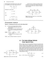
Figure C.16 A Experimental determination of the
ratio MfL
x
.
738
More
on Magnetically Coupled Coils and Ideal Transformers
In deriving the expressions for the inductances there, we used the
relationship M = kVL\L
2
. Expressing the inductances as functions of
the self-inductances L\ and L
2
and the coefficient of coupling k allows the

values of a given by Eqs. C.20 and C.21 not only to reduce the number of
inductances needed in the equivalent circuit, but also to guarantee that all
the inductances will be positive. We leave to you to investigate the conse-
quences of choosing the value of a given by Eq. C.22.
The values of a given by Eqs. C.20-C.22 can be determined experi-
mentally. The ratio MjL
x
is obtained by driving the coil designated as hav-
ing N\ turns by a sinusoidal voltage source. The source frequency is set
high enough that coL\ 5$> R\, and the N
2
coil is left open. Figure C.16
shows this arrangement.
With the N
2
coil open,
V
2
=
juiM\
{
.
(C.23)
Now, as /a>L] » R
h
the current I\ is
I. = 77
(
C
-

24
)
ja)L
[
Substituting Eq. C.24 into Eq. C23 yields
(C.25)
in which the ratio M/L
l
is the terminal voltage ratio corresponding to
coil 2 being open; that
is,
I
2
= 0.
We obtain the ratio L
2
/M by reversing the procedure; that is, coil 2 is
energized and coil
1
is left open. Then
Finally, we observe that the value of a given by Eq. C.22 is the geo-
metric mean of these two voltage ratios; thus
VxA-oVViA-o VL, M
(C.27)
For coils wound on nonmagnetic cores, the voltage ratio is not the
same as the turns ratio, as it very nearly is for coils wound on ferromagnetic
cores.
Because the self-inductances vary as the square of the number of
turns,
Eq. C27 reveals that the turns ratio is approximately equal to the

geometric mean of the two voltage ratios, or
Appendix
~L
'
D The Decibel
Telephone engineers who were concerned with the power loss across the
cascaded circuits used to transmit telephone signals introduced the deci-
bel.
Figure D.l defines the problem.
There, p, is the power input to the system, p
x
is the power output of
circuit A, p
2
is the power output of circuit B, and
p
(>
is the power output
of the system. The power gain of each circuit is the ratio of the power out
to the power in. Thus
Pi
P\
B
Pi
-# •-
C
P<>
Figure D.l • Three cascaded circuits.
P\
P2 , Pa

CTA = —, an = —, and err — —.
Pi Pi Pi
The overall power gain of the system is simply the product of the individ-
ual gains, or
Po
Pi
P^PlPo
Pi Pi Pi
= (T
A
<r
B
a
c
.
The multiplication of power ratios is converted to addition by means of
the logarithm; that is,
log
10
— = logujo-A + log
1()
o-
B
+ log
1()
cr
c
,
Pi
This log ratio of the powers was named the bel, in honor of Alexander

Graham Bell. Thus we calculate the overall power gain, in bels, simply by
summing the power gains, also in bels, of each segment of the transmission
system. In practice, the bel is an inconveniently large quantity. One-tenth
of a bel is a more useful measure of power gain; hence the decibel. The
number of decibels equals 10 times the number of bels, so
Po
Number of decibels = 10 login —
Pi
When we use the decibel as a measure of power ratios, in some situa-
tions the resistance seen looking into the circuit equals the resistance
loading the circuit, as illustrated in Fig. D.2.
When the input resistance equals the load resistance, we can convert
the power ratio to either a voltage ratio or a current ratio:
Po
Pi
v
ou\
Via
'in
'"in •*
A
'out
+-
+ {
R,
Figure D.2 • A circuit in which the input resistance
equals the load resistance.
or
Po
Pi

if
R
'in
739
740 The Decibel
These equations show that the number of decibels becomes
Number of decibels = 20
log]
0
'out
= 20 log
'out
10
(D.l)
TABLE D.l Some dB-Ratio Pairs
dB
0
3
6
10
15
20
Ratio
1.00
1.41
2.00
3.16
5.62
10.00
dB

30
40
60
80
100
120
Ratio
31.62
100.00
10
3
10
4
10
5
10
6
The definition of the decibel used in Bode diagrams (see Appendix E)
is borrowed from the results expressed by Eq. D.l, since these results
apply to any transfer function involving a voltage ratio, a current ratio, a
voltage-to-current ratio, or a current-to-voltage ratio. You should keep the
original definition of the decibel firmly in mind because it is of fundamen-
tal importance in many engineering applications.
When you are working with transfer function amplitudes expressed in
decibels, having a table that translates the decibel value to the actual value
of the output/input ratio is helpful. Table D.l gives some useful pairs. The
ratio corresponding to a negative decibel value is the reciprocal of the pos-
itive ratio. For example, -3 dB corresponds to an output/input ratio of
1/1.41, or 0.707. Interestingly,
—3

dB corresponds to the half-power fre-
quencies of the filter circuits discussed in Chapters 14 and 15.
The decibel is also used as a unit of power when it expresses the ratio
of a known power to a reference power. Usually the reference power is
1 mW and the power unit is written dBm, which stands for "decibels rela-
tive to one milliwatt." For example, a power of 20 mW corresponds to
±13 dBm.
AC voltmeters commonly provide dBm readings that assume not only
a 1 mW reference power but also a 600 ft reference resistance (a value
commonly used in telephone systems). Since a power of 1 mW in 600 ft
corresponds to 0.7746 V (mis), that voltage is read as 0 dBm on the meter.
For analog meters, there usually is exactly a 10 dB difference between
adjacent ranges. Although the scales may be marked 0.1,
0.3,1,
3,10, and
so on, in fact 3.16 V on the 3 V scale lines up with
1
V on the 1 V scale.
Some voltmeters provide a switch to choose a reference resistance (50,
135,600, or 900 ft) or to select dBm or dBV (decibels relative to one volt).
Appendix
Q Bode Diagrams
As we have seen, the frequency response plot is a very important tool for
analyzing a circuit's behavior. Up to this point, however, we have shown
qualitative sketches of the frequency response without discussing how to
create such diagrams. The most efficient method for generating and plot-
ting the amplitude and phase data is to use a digital computer; we can rely
on it to give us accurate numerical plots of \H(jm)\ and
d{ja>)
versus co.

However, in some situations, preliminary sketches using Bode diagrams
can help ensure the intelligent use of the computer.
A Bode diagram, or plot, is a graphical technique that gives a feel
for the frequency response of a circuit. These diagrams are named in
recognition of the pioneering work done by H.
W.
Bode.
1
They are most
useful for circuits in which the poles and zeros of H(s) are reasonably
well separated.
Like the qualitative frequency response plots seen thus far, a Bode
diagram consists of two separate plots: One shows how the amplitude of
H(jco) varies with frequency, and the other shows how the phase angle
of H(j(o) varies with frequency. In Bode diagrams, the plots are made on
semilog graph paper for greater accuracy in representing the wide range
of frequency values. In both the amplitude and phase plots, the frequency
is plotted on the horizontal log scale, and the amplitude and phase angle
are plotted on the linear vertical scale.
E,l Real, First-Order Poles and Zeros
To simplify the development of Bode diagrams, we begin by considering
only cases where all the poles and zeros of H(s) are real and first order.
Later we will present cases with complex and repeated poles and zeros.
For our purposes, having a specific expression for H(s) is helpful. Hence
we base the discussion on
K(s + zi)
from which
ui> \ ^O
+
*l)

]0)(j(0
+ Pi)
The first step in making Bode diagrams is to put the expression for
H(jco) in a standard form, which we derive simply by dividing out the
poles and zeros:
Kzi(l +/w/zi)
f s
H(m) = ,.
w<
. , (E.3)
p,(7a.)(l + /a>/A)
1
See II.
W.
Bode, Network Analysis and Feedback Design (New York: Van Nostrand, 1945).
742 Bode Diagrams
Next we let K
a
represent the constant quantity Kz.[/p\, and at the
same time we express H(jto) in polar form:
M /90 |1 + J^/Pil /j3i
K„|l + /w/zil
Mil + WAI
(E.4)
From Eq. E.4,
\H(ja>)\
= / ; ', (E.5)
0(«) = ?Ai - 90° - /3,. (E.6)
By definition, the phase angles
ip\

and /3j are
0, = tan ~
x
wfz\\ (E.7)
j3i = tan^w/Pi- (
E
-
8
)
The Bode diagrams consist of plotting Eq. E.5 (amplitude) and Eq. E.6
(phase) as functions of
o>.
E.2 Straight-Line Amplitude Plots
The amplitude plot involves the multiplication and division of factors
associated with the poles and zeros of H(s). We reduce this multiplication
and division to addition and subtraction by expressing the amplitude of
H(j(o) in terms of a logarithmic value: the decibel (dB).
2
The amplitude
of H(ja)) in decibels is
/l
tlB
= 2()log
1()
|//f>)|. (E.9)
TABLE E.1 Actual Amplitudes and Their
To
§
ive
y°

u a feel for the unit of
decibels, Table E.l provides a translation
Decibel Values between the actual value of several amplitudes and their values in deci-
bels.
Expressing Eq. E.5 in terms of decibels gives
K
0
\l+jco/
Zl
\
A
dB
= 20 log
J()
w|l + ja>/pi\
= 201og
1()
/C + 20lQg
t
Jl + /»/*il
- 20 log
10
<u - 20 log
10
|l -f- ja/pxl (E.10)
See Appendix
D
for more information regarding the decibel.
AiB
0

3
6
10
15
20
A
1.00
1.41
2.00
3.16
5.62
10.00
AiB
30
40
60
SO
100
120
A
31.62
100.00
10
3
10
4
10
5
10
6

The key to plotting Eq. E.10 is to plot each term in the equation sepa-
rately and then combine the separate plots graphically. The individual fac-
tors are easy to plot because they can be approximated in all cases by
straight lines.
The plot of 20 log
10
K
(>
is a horizontal straight line because K
0
is not a
function of frequency. The value of this term is positive for K
a
> 1, zero
for K
0
- 1, and negative for K
0
< 1.
Two straight lines approximate the plot of 20
log
10
|
1
+• j(o/z\\. For small
values of
<w,
the magnitude
11
+ jafz\

|
is approximately
1,
and therefore
201og
1()
|l + j(o/zi\^0 asw-^0.
(E.ll)
For large values of w, the magnitude |1 + jo)/z\\ is approximately o)/z\,
and therefore
201og
1()
|l +
j(o/z.[\
^20 \og
u)
((o/Z]) asw—>oc.
(E.12)
On a log frequency scale, 20 \og
m
(a)/z\) is a straight line with a slope of
20 dB/decade (a decade is a 10-to-l change in frequency).This straight
line intersects the 0 dB axis at w = z\. This value of o» is called the
corner frequency.Thus, on the basis of Eqs. E.ll and E.12, two straight
lines can approximate the amplitude plot of a first-order zero, as
shown in Fig. E.l.
The plot of — 201ogioa> is a straight line having a slope of
-20 dB/decade that intersects the 0 dB axis at a» = l.Two straight lines
approximate the plot of -20 log
10

|l 4- jco/p\\. Here the two straight lines
25
20
15
10
5
0
-5
z
z
()I
°8H.||T)
\y
20 dB/dec
- Uecade
ade
1C
Z)
1 2 3 4 5 6 7 8 910
o)
(rad/s)
20 30 40 50
Figure E.l •
A
straight-line approximation of the amplitude plot of
a
first-order zero.
intersect on the 0 dB axis at w = p\. For large values of
w,
the straight line

20 log
10
(o>/pi) has a slope of -20 dB/decade. Figure E.2 shows the
straight-line approximation of the amplitude plot of a first-order pole.
klB
5
0
-5
-10
-15
-20
p
N
Sj
201og
10
|j^j
•
-20 dB/decade ^\
iQPi
1 2 3 4 5 6 78910
o)
(rad/s)
20 30 40 50
Figure E.2 • A straight-line approximation of the amplitude plot of a first-order pole.
Figure E.3 shows a plot of Eq. E.10 for K
0
= VlO, Z\ = 0.1 rad/s,
and pi = 5 rad/s. Each term in Eq. E.10 is labeled on Fig. E.3, so you can
verify that the individual terms sum to create the resultant plot, labeled

201og
1()
|//(/a>)|.
Example E.l illustrates the construction of a straight-line amplitude
plot for a transfer function characterized by first-order poles and zeros.
A
dB
50
40
30
20
10
0
-10
-20
\
\
\
\
S
N
yl
\,
>
mi
0 log,
0
\
-1
N

\
/
/
•
\l
)1
S
>
s
III
(/«01
Jgio^
•
•
<• •
>
s
>
/
/
\
s
20
s
/
C
\
logio
^
V

s
\
s
/
***
*
•
K
0
V
.'1111
-201o
s *
\
01
I0\oi
\
ogio
\
;iol^C
^
i+/|
CO
)
J
\
1
j,
0.05
0.1

0.5 1.0 5 10 50 100 500
a>
(rad/s)
Figure E.3 • A straight-line approximation of the amplitude plot for Eq. E.10.
E.2 Straight-Line Amplitude Plots 745
Example E.l
For the circuit in Fig. E.4:
a) Compute the transfer function, H(s).
b) Construct a straight-line approximation of the
Bode amplitude plot.
c) Calculate 20log
10
|.//(/cu)| at w = 50 rad/s and
co = 1000 rad/s.
d) Plot the values computed in (c) on the straight-
line graph; and
e) Suppose that v
t
{t) = 5cos (500* + 15°) V, and
then use the Bode plot you constructed to pre-
dict the amplitude of v
a
(t) in the steady state.
100
mH
10
.mF
I
11
ill

V,
Figure
E.4 • The circuit for Example E.l.
c) We have
//(/50) =
o.ii(;50)
(1 + /5)(1 + /0.5)
Solution
a) Transforming the circuit in Fig. E.4 into the
s-domain and then using 5-domain voltage divi-
sion gives
= 0.9648/-15.25°,
20 log
10
|//(/50)| = 20 log
10
0.9648
H(s) =
(R/L)s
i
•
S* + (R/L)s + £
Substituting the numerical values from the cir-
cuit, we get
= -0.311 dB;
//(/1000) =
0.11(/1000)
(1 + /100)(1 + /10)
H(s) =
110s 1105

s
2
+ 110$ + 1000 (s + 10)(5 + 100)
b) We begin by writing H(jto) in standard form:
= 0.1094/-83.72°;
20 log
1()
0.1094 = -19.22 dB.
H(ja>) =
0.11;a»
[1 + /(a>/10)][l + /K100)]'
The expression for the amplitude of
H(J<&)
in
decibels is
A
dB
= 201og
1()
|//(/
w
)|
= 201og
10
0.11 + 201og
10
|H
-
20 log
10 1+/

-20 log
10
Figure E.5 shows the straight-line plot.
Each term contributing to the overall amplitude
is identified.
40
30
20
10
0
Am -10
-20
-30
-40
-50
-60
1 5 10 50 100 5001000
co
(rad/s)
Figure
E.5 • The straight-line amplitude plot for the transfer function of
the
circuit in Fig. E.4.
•*
,*"'
•
^20
lo
T
y

y
'"
^20'log
,.—
SloO.ll
imr
-15
"'s&
-
|
o
\M
\c
Ml
N
—0.311
WrA
NfFx
.
CO i
201og
10
|i
+y-
1
| i i
r i
mi
-1 2
.1

1 1
MINI
0
l0S,r
1 1
+ /
1
II
IIIII
10
log,
k,
)
*^i
-^.
__
v
CO
10
1
»\H(jco
ill
-fn
;l^<
T
S
*
S
N
>

i
1
N,
T
t
1""
5)
|
-19.22)"
V^
Yk
2s>.
_.l.