Basic Theoretical Physics: A Concise Overview P2 pptx

XII Contents
28.3 Unitary Equivalence; Change of Representation . . . . . . . . . . . . 245
29 Spin Momentum and the Pauli Principle
(Spin-statistics Theorem) 249
29.1 Spin Momentum;
the Hamilton Operator with Spin-orbit Interaction. . . . . . . . . . 249
29.2 Rotation of Wave Functions with Spin;
Pauli’s Exclusion Principle. . . . . . . . . . . . . . . . . . . . . . . . . . . . . . . 251
30 Addition of Angular Momenta 255
30.1 Composition Rules for Angular Momenta . . . . . . . . . . . . . . . . . . 255
30.2 Fine Structure of the p-Levels; Hyperfine Structure . . . . . . . . . 256
30.3 Vector Model of the Quantization of the Angular Momentum 257
31 Ritz Minimization 259
32 Perturbation Theory for Static Problems 261
32.1 FormalismandResults 261
32.2 Application I: Atoms in an Electric Field; The Stark Effect . . 263
32.3 Application II: Atoms in a Magnetic Field; Zeeman Effect . . . 264
33 Time-dependent Perturbations 267
33.1 Formalism and Results; Fermi’s “Golden Rules” . . . . . . . . . . . . 267
33.2 SelectionRules 269
34 Magnetism: An Essentially Quantum Mechanical
Phenomenon 271
34.1 Heitler and London’s Theory of the H
2
-Molecule 271
34.2 Hund’s Rule. Why is the O
2
-Molecule Paramagnetic? . . . . . . . 275
35 Cooper Pairs; Superconductors and Superfluids 277
36 On the Interpretation of Quantum Mechanics
(Reality?, Locality?, Retardation?) 279

36.1 Einstein-Podolski-RosenExperiments 279
36.2 The Aharonov-Bohm Effect; Berry Phases . . . . . . . . . . . . . . . . . 281
36.3 QuantumComputing 283
36.4 2dQuantumDots 285
36.5 Interaction-free Quantum Measurement;
“WhichPath?”Experiments 287
36.6 Quantum Cryptography 289
37 Quantum Mechanics: Retrospect and Prospect 293
38 Appendix: “Mutual Preparation Algorithm”
for Quantum Cryptography 297
Contents XIII
Part IV Thermodynamics and Statistical Physics
39 Introduction and Overview to Part IV 301
40 Phenomenological Thermodynamics:
Temperature and Heat 303
40.1 Temperature 303
40.2 Heat 305
40.3 Thermal Equilibrium and Diffusion of Heat . . . . . . . . . . . . . . . . 306
40.4 Solutionsofthe DiffusionEquation 307
41 The First and Second Laws of Thermodynamics 313
41.1 Introduction:Work 313
41.2 First and Second Laws: Equivalent Formulations . . . . . . . . . . . 315
41.3 Some Typical Applications: C
V
and
∂U
∂V
;
TheMaxwellRelation 316
41.4 GeneralMaxwellRelations 318

41.5 The Heat Capacity Differences C
p
− C
V
and C
H
− C
m
318
41.6 Enthalpy and the Joule-Thomson Experiment;
LiquefactionofAir 319
41.7 Adiabatic ExpansionofanIdealGas 324
42 Phase Changes, van der Waals Theory
and Related Topics 327
42.1 VanderWaals Theory 327
42.2 Magnetic Phase Changes; The Arrott Equation. . . . . . . . . . . . . 330
42.3 Critical Behavior; Ising Model; Magnetism and Lattice Gas . . 332
43 The Kinetic Theory of Gases 335
43.1 Aim 335
43.2 TheGeneralBernoulliPressureFormula 335
43.3 Formulafor PressureinanInteractingSystem 341
44 Statistical Physics 343
44.1 Introduction; Boltzmann-Gibbs Probabilities . . . . . . . . . . . . . . . 343
44.2 The Harmonic Oscillator and Planck’s Formula . . . . . . . . . . . . . 344
45 The Transition to Classical Statistical Physics 349
45.1 The Integral over Phase Space;
Identical Particles in Classical StatisticalPhysics 349
45.2 The Rotational Energy of a Diatomic Molecule . . . . . . . . . . . . . 350
XIV Contents
46 Advanced Discussion of the Second Law 353

46.1 FreeEnergy 353
46.2 On the Impossibility of Perpetual Motion
oftheSecond Kind 354
47 Shannon’s Information Entropy 359
48 Canonical Ensembles
in Phenomenological Thermodynamics 363
48.1 ClosedSystemsandMicrocanonicalEnsembles 363
48.2 The Entropy of an Ideal Gas
fromtheMicrocanonicalEnsemble 363
48.3 Systems in a Heat Bath:
Canonical and Grand Canonical Distributions . . . . . . . . . . . . . . 366
48.4 From Microcanonical to Canonical and Grand Canonical
Ensembles 367
49 The Clausius-Clapeyron Equation 369
50 Production of Low and Ultralow Temperatures;
Third Law 371
51 General Statistical Physics
(Statistical Operator; Trace Formalism) 377
52 Ideal Bose and Fermi Gases 379
53 Applications I: Fermions, Bosons,
Condensation Phenomena 383
53.1 ElectronsinMetals (SommerfeldFormalism) 383
53.2 Some Semiquantitative Considerations on the Development
ofStars 387
53.3 Bose-EinsteinCondensation 391
53.4 Ginzburg-Landau Theory of Superconductivity . . . . . . . . . . . . . 395
53.5 Debye Theoryofthe HeatCapacityofSolids 399
53.6 Landau’s Theory of 2nd-order Phase Transitions . . . . . . . . . . . 403
53.7 Molecular Field Theories; Mean Field Approaches . . . . . . . . . . 405
53.8 Fluctuations 408

53.9 MonteCarloSimulations 411
54 Applications II: Phase Equilibria in Chemical Physics 413
54.1 Additivity of the Entropy; Partial Pressure;
EntropyofMixing 413
54.2 ChemicalReactions;the LawofMassAction 416
54.3 Electron Equilibrium in Neutron Stars . . . . . . . . . . . . . . . . . . . . 417
54.4 Gibbs’PhaseRule 419
Contents XV
54.5 OsmoticPressure 420
54.6 Decrease of the Melting Temperature Due to “De-icing” Salt . 422
54.7 The Vapor Pressure of Spherical Droplets . . . . . . . . . . . . . . . . . 423
55 Conclusion to Part IV 427
References 431
Index 435
Part I
Mechanics and Basic Relativity
1 Space and Time
1.1 Preliminaries to Part I
This book begins in an elementary way, before progressing to the topic of an-
alytical mechanics.
1
Nonlinear phenomena such as “chaos” are treated briefly
in a separate chapter (Chap. 12). As far as possible, only elementary formulae
have been used in the presentation of relativity.
1.2 General Remarks on Space and Time
a) Physics is based on experience and experiment, from which axioms or gen-
erally accepted principles or laws of nature are developed. However, an
axiomatic approach, used for the purposes of reasoning in order to estab-
lish a formal deductive system, is potentially dangerous and inadequate,
since axioms do not constitute a necessary truth, experimentally.

b) Most theories are only approximate, preliminary, and limited in scope.
Furthermore, they cannot be proved rigorously in every circumstance (i.e.,
verified), only shown to be untrue in certain circumstances (i.e., falsified;
Popper).
2
For example, it transpires that Newtonian mechanics only ap-
pliesaslongasthemagnitudesofthevelocitiesoftheobjectsconsidered
are very small compared to the velocity c of light in vacuo.
c) Theoretical physics develops (and continues to develop) in “phases”
(Kuhn
3
, changes of paradigm). The following list gives examples.
1. From ∼ 1680−1860: classical Newtonian mechanics,falsifiedbyexper-
iments of those such as Michelson and Morley (1887). This falsification
was ground-breaking since it led Einstein in 1905 to the insight that
the perceptions of space and time, which were the basis of Newtonian
theory, had to be modified.
2. From ∼ 1860−1900: electrodynamics (Maxwell). The full consequences
of Maxwell’s theory were only later understood by Einstein through
his special theory of relativity (1905), which concerns both Newtonian
1
See, for example, [3].
2
Here we recommend an internet search for Karl Popper.
3
For more information we suggest an internet search for Thomas Samuel Kuhn.
4 1 Space and Time
mechanics (Part I) and Maxwell’s electrodynamics (Part II). In the
same year, through his hypothesis of quanta of electromagnetic waves
(photons), Einstein also contributed fundamentally to the developing

field of quantum mechanics (Part III).
3. 1905: Einstein’s special theory of relativity, and 1916: his general theory
of relativity.
4. From 1900: Planck, Bohr, Heisenberg, de Broglie, Schr¨odinger: quan-
tum mechanics; atomic and molecular physics.
5. From ∼1945: relativistic quantum field theories, quantum electro-
dynamics, quantum chromodynamics, nuclear and particle physics.
6. From ∼1980: geometry (spacetime) and cosmology: supersymmetric
theories, so-called ‘string’ and ‘brane’ theories; astrophysics; strange
matter.
7. From ∼1980: complex systems and chaos; nonlinear phenomena in
mechanics related to quantum mechanics; cooperative phenomena.
Theoretical physics is thus a discipline which is open to change. Even in
mechanics, which is apparently old-fashioned, there are many unsolved prob-
lems.
1.3 Space and Time in Classical Mechanics
Within classical mechanics it is implicitly assumed – from relatively inaccu-
rate measurements based on everyday experience – that
a) physics takes place in a three-dimensional Euclidean space that is not
influenced by material properties and physical events. It is also assumed
that
b) time runs separately as an absolute quantity; i.e., it is assumed that all
clocks can be synchronized by a signal transmitted at a speed v →∞.
Again, the underlying experiences are only approximate, e.g., that
α) measurements of lengths and angles can be performed by translation and
rotation of rigid bodies such as rods or yardsticks;
β) the sum of the interior angles of a triangle is 180
◦
, as Gauss showed in
his famous geodesic triangulation of 1831.

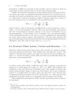
Thus, according to the laws of classical mechanics, rays of light travel in
straight lines (rectilinear behavior). Einstein’s prediction that, instead, light
could travel in curved paths became evident as a result of very accurate as-
tronomical measurements when in 1919 during a solar eclipse rays of light
traveling near the surface of the sun were observed showing that stellar bod-
ies under the influence of gravitation give rise to a curvature of spacetime
(general theory of relativity), a phenomenon which was not measurable in
Gauss’s time.
Assumption b) was also shown to be incorrect by Einstein (see below).
2 Force and Mass
2.1 Galileo’s Principle (Newton’s First Axiom)
Galileo’s principle, which forms the starting point of theoretical mechanics,
states that in an inertial frame of reference all bodies not acted upon by any
force move rectilinearly and homogeneously at constant velocity v.
The main difficulty arising here lies in the realization of an inertial frame,
which is only possible by iteration: to a zeroth degree of approximation an
inertial frame is a system of Cartesian coordinates, which is rigidly rotating
with the surface of the earth, to which its axes are attached; to the next
approximation they are attached to the center of the earth; in the following
approximation they are attached to the center of the sun, to a third approxi-
mation to the center of our galaxy, and so on. According to Mach an inertial
frame can thus only be defined by the overall distribution of the stars. The
final difficulties were only resolved later by Einstein, who proposed that in-
ertial frames can only be defined locally, since gravitation and acceleration
are equivalent quantities (see Chap. 14).
Galileo’s principle is essentially equivalent to Newton’s First Axiom (or
Newton’s First Law of Motion).
2.2 Newton’s Second Axiom:
Inertia; Newton’s Equation of Motion
This axiom constitutes an essential widening and accentuation of Galileo’s

principle through the introduction of the notions of force, F ,andinertial
mass, m
t
≡ m. (This is the inertial aspect of the central notion of mass, m.)
Newton’s second law was originally stated in terms of momentum. The
rate of change of momentum of a body is proportional to the force acting on
the body and is in the same direction. where the momentum of a body of
inertial mass m
t
is quantified by the vector p := m
t
·v.
1
Thus
F =
dp
dt
. (2.1)
1
Here we consider only bodies with infinitesimal volume: so-called point masses.
62ForceandMass
The notion of mass also has a gravitational aspect, m
s
(see below), where
m
t
= m
s
(≡ m). However, primarily a body possesses ‘inertial’ mass m
t

,
which is a quantitative measure of its inertia or resistance to being moved
2
.
(Note: In the above form, (2.1) also holds in the special theory of relativity,
see Sect. 15 below, according to which the momentum is given by
p =
m
0
v

1 −
v
2
c
2
;
m
0
is the rest mass, which only agrees with m
t
in the Newtonian approxi-
mation v
2
 c
2
,wherec is the velocity of light in vacuo.)
Equation (2.1) can be considered to be essentially a definition of force
involving (inertial) mass and velocity, or equivalently a definition of mass in
terms of force (see below).

As already mentioned, a body with (inertial) mass also produces a gravi-
tational force proportional to its gravitational mass m
s
. Astonishingly, in
the conventional units, i.e., apart from a universal constant, one has the
well-known identity m
s
≡ m
t
, which becomes still more astonishing, if one
simply changes the name and thinks of m
s
as a “gravitational charge” instead
of “gravitational mass”. This remarkable identity, to which we shall return
later, provided Einstein with strong motivation for developing his general
theory of relativity.
2.3 Basic and Derived Quantities; Gravitational Force
The basic quantities underlying all physical measurements of motion are
– time: defined from multiples of the period of a so-called ‘atomic clock’,
and
– distance: measurements of which are nowadays performed using radar
signals.
The conventional units of time (e.g., second, hour, year) and length (e.g.,
kilometre, mile, etc.) are arbitrary. They have been introduced historically,
often from astronomical observations, and can easily be transformed from
one to the other. In this context, the so-called “archive metre” (in French:
“m`etre des archives”) was adopted historically as the universal prototype for
a standard length or distance: 1 metre (1 m).
Similarly, the “archive kilogram” or international prototype kilogram in
Paris is the universal standard for the unit of mass: 1 kilogram (1 kg).

2
in German: inertial mass = tr¨age Masse as opposed to gravitational mass =
schwere Masse m
s
. The fact that in principle one should distinguish between
the two quantities was already noted by the German physicist H. Hertz in 1884;
see [4].
2.3 Basic and Derived Quantities; Gravitational Force 7
However, the problem as to whether the archive kilogram should be used
as a definition of (inertial) mass or a definition of force produced a dilemma.
In the nineteen-fifties the “kilopond (kp)” (or kilogram-force (kgf)) was
adopted as a standard quantity in many countries. This quantity is defined
as the gravitational force acting on a 1 kg mass in standard earth gravity (in
Paris where the archive kilogram was deposited). At that time the quantity
force was considered to be a “basic” quantity, while mass was (only) a “de-
rived” one. More recently, even the above countries have reverted to using
length, time,and(inertial) mass as base quantities and force as a derived
quantity. In this book we shall generally use the international system (SI)
of units, which has 7 dimensionally independent base units: metre, kilogram,
second, ampere, kelvin, mole and candela. All other physical units can be
derived from these base units.
What can be learnt from this? Whether a quantity is basic or (only) de-
rived,isamatter of convention.Eventhenumber of base quantities is not
fixed; e.g., some physicists use the ‘cgs’ system, which has three base quan-
tities, length in centimetres (cm), time in seconds (s) and (inertial) mass in
grams (g), or multiples thereof; or the mksA system, which has four base
quantities, corresponding to the standard units: metre (m), kilogram (kg),
second (s) and ampere (A) (which only comes into play in electrodynamics).
Finally one may adopt a system with only one basic quantity, as preferred
by high-energy physicists, who like to express everything in terms of a funda-

mental unit of energy, the electron-volt eV: e.g., lengths are expressed in units
of  ·c/(eV), where  is Planck’s constant divided by 2π, which is a universal
quantity with the physical dimension action = energy ×time, while c is the
velocity of light in vacuo; masses are expressed in units of eV/c
2
,whichisthe
“rest mass” corresponding to the energy 1 eV. (Powers of  and c are usually
replaced by unity
3
).
As a consequence, writing Newton’s equation of motion in the form
m · a = F (2.2)
(relating acceleration a :=
d
2
r
dt
2
and force F ), it follows that one can equally
well say that in this equation the force (e.g., calibrated by a certain spring)
is the ‘basic’ quantity, as opposed to the different viewpoint that the mass
is ‘basic’ with the force being a derived quantity, which is ‘derived’ by the
above equation. (This arbitariness or dichotomy of viewpoints reminds us of
the question: “Which came first, the chicken or the egg?!”). In a more modern
didactical framework based on current densities one could, for example, write
the left-hand side of (2.2) as the time-derivative of the momentum,
dp
dt
≡
F , thereby using the force as a secondary quantity. However, as already

3
One should avoid using the semantically different formulation “set to 1” for the
quantities with non-vanishing physical dimension such as c(= 2.998 · 10
8
m/s),
etc.