Basic Theoretical Physics: A Concise Overview P3 pdf

82ForceandMass
mentioned, a different viewpoint is also possible, and it is better to keep an
open mind on these matters than to fix our ideas unnecessarily.
Finally, the problem of planetary motion dating back to the time of New-
ton where one must in principle distinguish between the inertial mass m
t
entering (2.2) and a gravitational mass m
s
, which is numerically identical to
m
t
(apart from a universal constant, which is usually replaced by unity), is
far from being trivial; m
s
is defined by the gravitational law:
F (r)=−γ
M
s
· m
s
|r − R|
2
·
r −R
|r − R|
,
where r and m
s
refer to the planet, and R and M
s
to the central star (“sun”),

while γ is the gravitational constant. Here the [gravitational] masses play
the role of gravitational charges, similar to the case of Coulomb’s law in
electromagnetism. In particular, as in Coulomb’s law, the proportionality
of the gravitational force to M
s
and m
s
can be considered as representing
an active and a passive aspect of gravitation.
4
The fact that inertial and
gravitational mass are indeed equal was first proved experimentally by E¨otv¨os
(Budapest, 1911 [6]); thus we may write m
s
= m
t
≡ m.
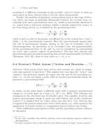
2.4 Newton’s Third Axiom (“Action and Reaction . . . ”)
Newton’s third axiom states that action and reaction are equal in magni-
tude and opposite in direction.
5
This implies inter alia that the “active” and
“passive” gravitational masses are equal (see the end of the preceding sec-
tion), i.e., on the one hand, a body with an (active) gravitational charge M
s
generates a gravitational field
G(r)=−γ
M
s
|r − R|

2
·
r −R
|r − R|
,
in which, on the other hand, a different body with a (passive) gravitational
charge m
s
is acted upon by a force, i.e., F = m
s
· G(r). The relations are
analogous to the electrical case (Coulomb’s law). The equality of active and
passive gravitational charge is again not self-evident, but in the considered
context it is implied that no torque arises (see also Sect. 5.2). Newton also
recognized the general importance of his third axiom, e.g., with regard to the
application of tensile stresses or compression forces between two bodies.
Three additional consequences of this and the preceding sections will now
be discussed.
4
If one only considers the relative motion, active and passive aspects cannot be
distinguished.
5
In some countries this is described by the abbreviation in Latin “actio=reactio”.
2.4 Newton’s Third Axiom (“Action and Reaction ”) 9
a) As a consequence of equating the inertial and gravitational masses in
Newton’s equation F (r)=m
s
·G(r)itfollowsthatall bodies fall equally
fast (if only gravitational forces are considered), i.e.: a(t)=G(r(t)).
This corresponds to Galileo’s experiment

6
,orratherthought experiment,
of dropping different masses simultanously from the top of the Leaning
Tower of Pisa.
b) The principle of superposition applies with respect to gravitational forces:
G(r)=−γ

k
(ΔM
s
)
k
|r − R
k
|
2
·
r −R
k
|r −R
k
|
.
Here (ΔM
s
)
k
:= 
k
ΔV

k
is the mass of a small volume element ΔV
k
,and

k
is the mass density. An analogous “superposition principle” also applies
for electrostatic forces, but, e.g., not to nuclear forces. For the principle
of superposition to apply, the equations of motion must be linear.
c) Gravitational (and Coulomb) forces act in the direction of the line joining
the point masses i and k. This implies a different emphasis on the meaning
of Newton’s third axiom. In its weak form, the postulate means that
F
i,k
= −F
k,i
; in an intensified or “strong” form it means that F
i,k
=
(r
i
−r
k
) ·f(r
i,k
), where f(r
ik
) is a scalar function of the distance r
i,k
:=

|r
i
− r
k
|.
As we will see below, the above intensification yields a sufficient condition
that Newton’s third axiom not only implies F
i,k
= −F
k,i
, but also D
i,k
=
−D
k,i
,whereD
i,k
is the torque acting on a particle at r
i
by a particle at r
k
.
6
In essence, the early statement of Galileo already contained the basis not only of
the later equation m
s
= m
t
, but also of the E¨otv¨os experiment, [6] (see also [4]),
and of Einstein’s equivalence principle (see below).

3 Basic Mechanics of Motion
in One Dimension
3.1 Geometrical Relations for Curves in Space
In this section, motion is considered to take place on a fixed curve in
three-dimensional Euclidean space. This means that it is essentially one-
dimensional; motion in a straight line is a special case of this.
For such trajectories we assume they are described by the radius vector
r(t), which is assumed to be continuously differentiable at least twice, for
t ∈ [t
a
,t
b
](wheret
a
and t
b
correspond to the beginning and end of the
motion, respectively). The instantaneous velocity is
v(t):=
dr
dt
,
and the instantaneous acceleration is
a(t):=
dv
dt
=
d
2
r

dt
2
,
where for convenience we differentiate all three components, x(t), y(t)and
z(t) in a fixed Cartesian coordinate system,
r(t)=x(t)e
x
+ y(t)e
y
+ z(t)e
z
:
dr(t)
dt
=˙x(t)e
x
+˙y(t)e
y
+˙z(t)e
z
.
For the velocity vector we can thus simply write: v(t)=v(t)τ (t), where
v(t)=

(˙x(t))
2
+(˙y(t))
2
+(˙z(t))
2

is the magnitude of the velocity and
τ (t):=
v(t)
|v(t)|
the tangential unit vector to the curve (assuming v =0).
v(t)andτ (t)arethusdynamical and geometrical quantities, respectively,
with an absolute meaning, i.e., independent of the coordinates used.
In the following we assume that τ (t) is not constant; as we will show, the
acceleration can then be decomposed into, (i), a tangential component, and,
12 3 Basic Mechanics of Motion in One Dimension
(ii), a normal component (typically: radially inwards), which has the direction
of a so-called osculating normal n to the curve, where the unit vector n is
proportional to
dτ
dt
, and the magnitude of the force (ii) corresponds to the
well-known “centripetal” expression
v
2
R
(see below); the quantity R in this
formula is the (instantaneous) so-called radius of curvature (or osculating
radius) and can be evaluated as follows:
1
R
= |
dτ
v ·dt
| .
1

Only the tangential force, (i), is relevant at all, whereas the centripetal
expression (ii) is compensated for by forces of constraint
2
, which keep the
motion on the considered curve, and need no evaluation except in special
instances.
The quantity
t

t
a
v(t)dt
is called the arc length s(t), with the differential ds := v(t)dt.Asalready
mentioned, the centripetal acceleration, directed towards the center of the
osculating circle,isgivenby
a
centrip.
.(t)=n(t)
v
2
(t)
R(t)
.
We thus have
a(t) ≡ τ (t) ·
dv(t)
dt
+ a
centrip.
(t) .

The validity of these general statements can be illustrated simply by con-
sidering the special case of circular motion at constant angular velocity, i.e.,
r(t):=R · (cos(ωt)e
x
+sin(ωt)e
y
) .
The tangential vector is
τ (t)=−sin(ωt)e
x
+cos(ωt)e
y
,
and the osculating normal is
n(t)=−(cos(ωt)e
x
+sin(ωt)e
y
) ,
i.e., directed towards the center. The radius of curvature R(t)isofcourse
identical with the radius of the circle. The acceleration has the above-
mentioned magnitude, Rω
2
= v
2
/R, directed inwards.
1
It is strongly recommended that the reader should produce a sketch illustrating
these relations.
2

This is a special case of d’Alembert’s principle, which is described later.
3.2 One-dimensional Standard Problems 13
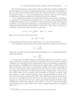
Fig. 3.1. Osculating circle and radius of curvature. The figure shows as a typical
example the lower part of an ellipse (described by the equation
y
1
b
:= 1 ±
q
1 −
x
2
a
2
,
with a := 2 and b := 1) and a segment (the lower of the two curves!) of the osculating
circle at x =0(withR :=
a
2
b
≡ 4). Usually a one-dimensional treatment suffices,
since an infinity of lines have the same osculating circle at a given point, and since
usually one does not require the radial component n ·
mv
2
R
of the force (which
is compensated by forces of constraint), as opposed to the tangential component
F
tangent

:= m · ˙v(t) ·τ (t)(wheret is the time, m the inertia and v the magnitude of
the considered point mass); n and τ are the osculating normal and the tangential
unit vectors, respectively. A one-dimensional treatment follows
Finally, as already alluded to above, the quanties τ(t), n(t), R(t), and s(t)
have purely geometrical meaning; i.e., they do not change due to the kine-
matics of the motion, but only depend on geometrical properties of the curve
on which the particle moves. The kinematics are determined by Newton’s
equations (2.2), and we can specialize these equations to a one-dimensional
problem, i.e., for ∼ τ (t), since (as mentioned) the transverse forces, n(t) ·
v
2
R
,
are compensated for by constraining forces.
The preceding arguments are supported by Fig. 3.1 above.
Thus, for simplicity we shall write x(t) instead of s(t) in the following,
and we have
v(t)=
dx(t)
dt
and m ·a(t)=m ·
d
2
x(t)
dt
2
= F (t, v(t),a(t)) ,
where F is the tangential component of the force, i.e., F ≡ F · τ .
3.2 One-dimensional Standard Problems
In the following, for simplicity, instead of F we consider the reduced quantity

f :=
F
m
.Iff(t, v, x) depends on only one of the three variables t, v or x,the
14 3 Basic Mechanics of Motion in One Dimension
equations of motion can be solved analytically. The most simple case is where
f is a function of t. By direct integration of
d
2
x(t)
dt
2
= f(t)
one obtains:
v(t)=v
0
+

t
t
0
d
˜
tf(
˜
t)andx(t)=x
0
+ v
0
·(t −t

0
)+

t
t
0
d
˜
tv(
˜
t) .
(x
0
, v
0
and t
0
are the real initial values of position, velocity and time.)
Thenextmostsimplecaseiswheref is given as an explicit function of v.
In this case a standard method is to use separation of variables (ˆ= transition
to the inverse function), if possible: Instead of
dv
dt
= f(v)
one considers
dt =
dv
f(v)
, or t − t
0

=

v
v
0
d˜v
f(˜v)
.
One obtains t as a function of v, and can thus, at least implicitly, calculate
v(t) and subsequently x(t).
The third case is where f ≡ f(x). In this case, for one-dimensional prob-
lems, one always proceeds using the principle of conservation of energy, i.e.,
from the equation of motion,
m
dv
dt
= F (x) ,
by multiplication with
v =
dx
dt
and subsequent integration, with the substitution v dt =dx, it follows that
v
2
2m
+ V (x) ≡ E
is constant, with a potential energy
V (x):=−
x


x
0
d˜xF (˜x) .
Therefore,
v(x)=

2
m
(E −V (x)) ,
3.2 One-dimensional Standard Problems 15
or dt =
dx

2
m
(E − V (x))
, and finally
t −t
0
=

x
x
0
d˜x

2
m
(E −V (˜x))
.

This relation is very useful, and we shall return to it often later.
If f depends on two or more variables, one can only make analytical
progress in certain cases, e.g., for the driven harmonic oscillator, with damp-
ing proportional to the magnitude of the velocity. In this important case,
which is treated below, one has a linear equation of motion, which makes the
problem solvable; i.e.,
¨x = −ω
2
0
x −
2
τ
v + f(t) ,
where useful general statements canbemade(seebelow).(Theabove-
mentioned ordinary differential equation applies to harmonic springs with
a spring constant k and mass m, corresponding to the Hookean force
F
H
:= −k · x,whereω
2
0
= k/m,plusalinear frictional force F
R
:= −m
2
τ
· v,
plus a driving force F
A
:= m · f(t).)

There are cases where the frictional force depends quadratically on the
velocity (so-called Newtonian friction),
F
R
:= −α ·
mv
2
2
,
i.e., with a so-called technical friction factor α, and a driving force depending
mainly, i.e., explicitly, on x, and only implicitly on t, e.g., in motor racing,
where the acceleration may be very high in certain places, F
a
= mf(x). The
equation of motion,
m ˙v = −α
mv
2
2
+ mf(x) ,
can then be solved by multiplying by
dt
dx

≡
1
v

:
One thus obtains the ordinary first-order differential equation

dv
dx
+
αv
2
=
f(x)
v
,
which can be solved by iteration. On the r.h.s. of this equation, one uses, for
example, an approximate expression for v(x) and obtains a refinement on the
l.h.s., which is then substituted into the r.h.s., etc., until one obtains con-
vergence. In almost all other cases one has to solve an ordinary second-order
differential equation numerically. Many computer programs are available for
solving such problems, so that it is not necessary to go into details here.
4 Mechanics of the Damped
and Driven Harmonic Oscillator
In this section the potential energy V (x) for the motion of a one-dimensional
system is considered, where it is assumed that V (x)issmootheverywhere
and differentiable an arbitrarily often number of times, and that for x =0,
V (x) has a parabolic local minimum. In the vicinity of x = 0 one then obtains
the following Taylor expansion, with V

(0) > 0:
V (x)=V (0) +
1
2
V

(0)x

2
+
1
3!
V

(0) x
3
+ ,
i.e.,
V (x)=V (0) +
mω
2
0
2
x
2
+ O

x
3

,
with ω
2
0
:= V

(0)/m, neglecting terms of third or higher order. For small os-
cillation amplitudes we thus have the differential equation of a free harmonic

oscillator of angular frequency ω
0
:
m¨x = −
dV
dx
, ¨x = −ω
2
x,
whose general solution is: x(t)=x
0
·cos(ω
0
t−α), with arbitrary real quantities
x
0
and α.
In close enough proximity to a parabolic local potential energy minimum,
one always obtains a harmonic oscillation (whose frequency is given by ω
0
:=
V

(0)
m
).
If one now includes (i) a frictional force, F
R
:= −γv, which can be char-
acterized by a so-called “relaxation time” τ (i.e., γ =: m · 2/τ), and (ii)

a driving force F
A
(t)=m · f(t), then one obtains the ordinary differential
equation
¨x +
2
τ
˙x + ω
2
0
x = f(t) .
This is a linear ordinary differential equation of second order (n ≡ 2) with
constant coefficients. For f (t) ≡ 0 this differential equation is homogeneous,
otherwise it is called inhomogeneous. (For arbitrary n =1, 2, the general
inhomogeneous form is:

d
n
d
n
t
+
n−1

ν=0
a
ν
d
ν
d

ν
t

x(t)=f(t)).
18 4 Mechanics of the Damped and Driven Harmonic Oscillator
For such differential equations, or for linear equations in general, the
principle of superposition applies: The sum of two solutions of the homo-
geneous equation, possibly weighted with real or complex coefficients, is also
a solution of the homogeneous equation; the sum of a “particular solution”
of the inhomogeneous equation plus an “arbitrary solution” of the homoge-
neous equation yields another solution of the inhomogeneous equation for
the same inhomogeneity; the sum of two particular solutions of the inhomo-
geneous equation for different inhomogeneities yields a particular solution
of the inhomogeneous differential equation, i.e., for the sum of the inhomo-
geneities.
The general solution of the inhomogeneous differential equation is there-
fore obtained by adding a relevant particular solution of the inhomogeneous
(i.e., “driven”) equation of motion to the general solution of the homogeneous
equation, i.e., the general “free oscillation”.
As a consequence, in what follows we shall firstly treat a “general free
oscillation”, and afterwards the seemingly rather special, but actually quite
general “periodically driven oscillation”, and also the seemingly very special,
but actually equally general so-called “ballistically driven oscillation”.
The general solution of the equation for a free oscillation, i.e., the general
solution of

d
n
d
n

t
+
n−1

ν=0
a
ν
d
ν
d
ν
t

x(t)=0 for n =2,
is obtained by linear combination of solutions of the form x(t) ∝ e
λ·t
.After
elementary calculations we obtain:
x(t)=exp

−
t
τ

·
⎧
⎨
⎩
x
0

cos


ω
2
0
−
1
τ
2
· t

+

v
0
+
x
0
τ

·
sin


ω
2
0
−
1

τ
2
· t


ω
2
0
−
1
τ
2
⎫
⎪
⎬
⎪
⎭
. (4.1)
This expression only looks daunting at first glance, until one realizes that the
bracketed expression converges for t → 0to
x
0
+

v
0
+
x
0
τ


· t,
as it must do.
Equation (4.1) applies not only for real
ε =

ω
2
0
−
1
τ
2
4 Mechanics of the Damped and Driven Harmonic Oscillator 19
but also for imaginary values, because in the limit t → 0 not only
sin(εt)
ε
,
but also
sin iεt
iε
→ t ;
x
0
and v
0
are the initial position and the initial velocity, respectively. Thus
the above-mentioned formula applies
a) not only for damped oscillations, i.e., for ε>0, or
ω

2
0
>
1
τ
2
,
i.e., sine or cosine oscillations with frequency
ω
1
:=

ω
2
0
−
1
τ
2
and the damping factor e
−λ
1
t
,withλ
1
:=
1
τ
,
b) but also for the aperiodic case,

ω
2
0
<
1
τ
2
,
since for real
ε :
sin(iε · t)
iε
≡ sinh εt , with
sinh(x):=
1
2
(e
x
− e
−x
) , and
cos(iεt) ≡ cosh(εt) , with
cosh(x):=
1
2
(e
x
+e
−x
):

In the aperiodic case, therefore, an exponential behavior with two char-
acteristic decay frequencies results (“relaxation frequencies”),
λ
±
:=
1
τ
±

1
τ
2
−
1
ω
2
0
.
Of these two relaxation frequencies the first is large, while the second is
small.
c) Exactly in the limiting case, ε ≡ 0, the second expression on the r.h.s.
of equation (4.1) is simply (v
0
+
x
0
τ
) ·t for all t, i.e., one finds the fastest
decay.