Basic Theoretical Physics: A Concise Overview P5 potx

32 6 Motion in a Central Force Field; Kepler’s Problem
6.2 Kepler’s Three Laws of Planetary Motion
They are:
1) The planets orbit the central star, e.g., the sun, on an elliptical path,where
the sun is at one of the two foci of the ellipse.
2) The vector from the center of the sun to the planet covers equal areas in
equal time intervals.
3) The ratio T
2
/a
3
,whereT is the time period and a the major principal
axis of the ellipse, is constant for all planets (of the solar system). (In
his famous interpretation of the motion of the moon as a planet orbiting
the earth, i.e., the earth was considered as the “central star”, Newton
concluded that this constant parameter is not just a universal number,
but proportional to the mass M of the respective central star.)
As already mentioned, Kepler’s second law is also known as the law of
equal areas and is equivalent to the angular momentum theorem for relative
motion, because (for relative motion
1
)
dL
dt
= r × F ,
i.e., ≡ 0 for central forces, i.e., if F ∼ r.Infact,wehave
L = r × p = m · r
2
˙ϕe
z
.

Here m is the reduced mass appearing in Newton’s equation for the rela-
tive motion of a “two-particle system” (such as planet–sun, where the other
planets are neglected); this reduced mass,
m
1+
m
M
,
is practically identical to the mass of the planet, since m  M .
The complete law of gravitation follows from Kepler’s laws by further
analysis which was first performed by Newton himself. The gravitational
force F ,whichapointmassM at position R
M
exerts on another point mass
m at r is given by:
F (r) ≡−γ
(m · M) ·(r − R
M
)
|r −R
M
|
3
. (6.2)
The gravitational force, which acts in the direction of the line joining r and
R
M
,is(i)attractive (since the gravitional constant γ is > 0), (ii) ∝ m · M,
and (iii) (as Coulomb’s law in electromagnetism) inversely proportional to
the square of the separation.

1
We do not write down the many sub-indices
rel.
, which we should use in principle.
6.3 Newtonian Synthesis: From Newton’s Theoryof Gravitation to Kepler 33
As has already been mentioned, the principle of superposition applies to
Newton’s law of gravitation with regard to summation or integration over
M, i.e., Newton’s theory of gravity, in contrast to Einstein’s general theory of
relativity (which contains Newton’s theory as a limiting case) is linear with
respect to the sources of the gravitational field.
Newton’s systematic analysis of Kepler’s laws (leading him to the impor-
tant idea of a central gravitational force) follows below; but firstly we shall
discuss the reverse path, the derivation (synthesis) of Kepler’s laws from New-
ton’s law of gravitation, (6.2). This timeless achievement of Newtonian theory
was accomplished by using the newly developed (also by Newton himself
2
)
mathematical tools of differential and integral calculus.
For 200 years, Newton was henceforth the ultimate authority, which makes
Einstein’s accomplishments look even greater (see below).
6.3 Newtonian Synthesis: From Newton’s Theory
of Gravitation to Kepler
Since in a central field the force possesses only a radial component, F
r
,(here
depending only on r, but not on ϕ), we just need the equation
m ·

¨r −r ˙ϕ
2


= F
r
(r) .
The force is trivially conservative, i.e.,
F = −gradV (r) ,
with potential energy
V (r) ≡−

r
∞
d˜rF
r
(˜r) .
Thus we have conservation of the energy:
m
2
·

˙r
2
+ r
2
˙ϕ
2

+ V (r)=E. (6.3)
Further, with the conservation law for the angular momentum we can elimi-
nate the variable ˙ϕ and obtain
m

2
· ˙r
2
+
L
2
2mr
2
+ V (r)=E. (6.4)
Here we have used the fact that the square of the angular momentum
(L = r × p)
2
Calculus was also invented independently by the universal genius Wilhelm Leib-
niz, a philosopher from Hanover, who did not, however, engage in physics.
34 6 Motion in a Central Force Field; Kepler’s Problem
is given by
3
the following relation:
L
2
=(mr
2
˙ϕ)
2
.
Equation (6.4) corresponds to a one-dimensional motion with an effective
potential energy
V
eff
(r):=V (r)+

L
2
2mr
2
.
The one-dimensional equation can be solved using the above method based
on energy conservation:
t − t
0
=
r

r
0
d˜r

2
m
(E − V
eff
(˜r))
.
Similarly we obtain from the conservation of angular momentum:
t −t
0
=
m
L
ϕ


ϕ
0
r
2
(˜ϕ) ·d˜ϕ.
Substituting
dt =

d˜ϕ
dt

−1
· d˜ϕ
we obtain:
ϕ(r)=ϕ
0
+
L
m
r

r
0
d˜r
˜r
2

2
m
(E − V

eff
(˜r))
. (6.5)
All these results apply quite generally. In particular we have used the fact
that the distance r depends (via t) uniquely on the angle ϕ,andvice versa,
at least if the motion starts (with ϕ = ϕ
0
=0)atthepointclosesttothe
central star, the so-called perihelion, and ends at the point farthest away, the
so-called aphelion.
6.4 Perihelion Rotation
What value of ϕ is obtained at the aphelion? It is far from being trivial (see
below) that this angle is exactly π, so that the planet returns to the perihelion
exactly after 2π. In fact, this is (almost) only true for Kepler potentials, i.e.,
for V = −A/r,whereA is a constant
4
, whereas (6.4) applies for more general
potentials that only depend on r. If these potentials deviate slightly from
3
In quantum mechanics we have L
2
→ 
2
l · (l + 1), see Part III.
4
We write “almost”, because the statement is also true for potentials ∝ r.
6.4 Perihelion Rotation 35
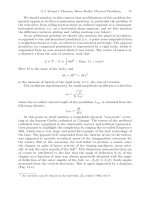
Fig. 6.1. Perihelion rotation. The function
r(t)=0.5/(1+0.5cos(2πt)) is plotted together
with the three straight lines: ϕ(t)=(2π)∗(1+

ε) ∗ t,withε = −0.1, 0.0and+0.1. The three
corresponding orbits r(φ) yield a closed ellipse
only for ε ≡ 0; in the other two cases one ob-
tains so-called rosette orbits, see the following
figure
the Kepler potential, one actually observes the phenomenon of perihelion
rotation, i.e., the aphelion position is not obtained for ϕ = π, but later (or
earlier), viz for
ϕ = π ±
1
2
Δϕ,
and the planet returns to the perihelion distance only at an angle deviating
from 2π, viz at 2π ±Δϕ, see Fig. 6.1 below.
Such a perihelion rotation is actually observed, primarily for the planet
Mercury which is closest to the sun. The reasons, all of them leading to tiny,
but measurable deviations from the -A/r-potential, are manifold, for example
– perturbations by the other planets and/or their moons can be significant,
– also deviations from the exact spherical shape of the central star may be
important,
– finally there are the general relativistic effects predicted by Einstein, which
have of course a revolutionary influence on our concept of space and time.
(Lest we forget, this even indirectly became a political issue during the
dark era of the Nazi regime in Germany during the 1930s.)
How perihelion rotation comes about is explained in Figs. 6.1 and 6.2.
In the following section we shall perform an analysis of Kepler’s laws,
analogously to Newtonian analysis, in order to obtain the laws of gravitation.
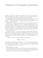
Fig. 6.2. Rosette orbits. If r(t)andϕ(t)
have different periods (here r(t)=0.5/(1 +
0.5cos(2πt)) but ϕ(t)=1.9π · t), one obtains

the rosette orbit shown. It corresponds exactly
to a potential energy of the non-Keplerian form
V (r)=−A/r − B/r
2
, and although looking
more complicated, it consists of only one con-
tinuous line represented by the above function
36 6 Motion in a Central Force Field; Kepler’s Problem
6.5 Newtonian Analysis: From Kepler’s Laws
to Newtonian Gravitation
As mentioned above, Newton used a rather long but systematic route to
obtain his law of gravitation,
F (r)=−γ
˜mM
r
2
r
r
,
from Kepler’s laws.
6.5.1 Newtonian Analysis I: Law of Force from Given Orbits
If the orbits are of the form
1
r
= f(ϕ), then one obtains by straightforward
differentiation:
−
˙r
r
2

=˙ϕ ·
d
dϕ
f(ϕ)=

L
mr
2

·
df
dϕ
, or
˙r = −
L
m
df
dϕ
, i.e.,
¨r = − ˙ϕ
L
m
d
2
f
dϕ
2
= −
L
2

m
2
r
2
d
2
f
dϕ
2
,
or finally the law of force:
F
r
m
≡ ¨r − r ˙ϕ
2
= −
L
2
m
2
r
2

d
2
f
dϕ
2
+

1
r

. (6.6)
Equation (6.6) will be used later.
6.5.2 Newtonian Analysis II: From the String Loop Construction
of an Ellipse to the Law F
r
= −A/r
2
Reminding ourselves of the elementary method for drawing an ellipse using
a loop of string, we can translate this into the mathematical expression
r + r

= r +

r
2
+(2a)
2
− 2r · 2e · cos ϕ
!
=2a.
Here 2a is the length of the major axis of the ellipse (which extends from
x = −a to x =+a for y ≡ 0); r and r

are the distances from the two foci
(the ends of the loop of string) which are situated at x = ±e on the major
axis,thex-axis, and ϕ is the azimuthal angle, as measured e.g., from the
6.5 Newtonian Analysis: From Kepler’s Laws to Newtonian Gravitation 37

left focus.
5
From this we obtain the parametric representation of the ellipse,
which was already well-known to Newton:
r =
p
1 − ε cos ϕ
,
or
1
r
=
1
p
·(1 −ε cos ϕ) . (6.7)
Here a
2
− e
2
=: b
2
,and
b
2
a
= p; b is the length of the minor semiaxis of the
ellipse. The parameter p is the distance from the left focus to the point of
the ellipse corresponding to the azimuthal angle ϕ =
π
2

,and
ε :=
a
2
− b
2
a
2
is the ellipticity,0≤ ε<1.
As a result of the above relations we already have the following inverse-
square law of force:
F
r
(r)=
−A
r
2
, where A>0
(attractive interaction), while the parameter p and the angular momen-
tum L are related to A by:
p =
L
2
A ·m
.
6.5.3 Hyperbolas; Comets
Equation (6.7) also applies where ε ≥ 1. In this case the orbits are no longer
ellipses (or circles, as a limiting case), but hyperbolas (or parabolas, as a lim-
iting case).
6

Hyperbolic orbits in the solar system apply to the case of nonreturning
comets, where the sun is the central point of the hyperbola, i.e., the perihe-
lion exists, but the aphelion is replaced by the limit r →∞. For repulsive
interactions, A<0, one would only have hyperbolas.
5
Here we recommend that the reader makes a sketch.
6
For the hydrogen atom the quantum mechanical case of continuum states at
E>0 corresponds to the hyperbolas of the Newtonian theory, whereas the
ellipses in that theory correspond to the bound states of the quantum mechanical
problem; see Part III of this volume.
38 6 Motion in a Central Force Field; Kepler’s Problem
6.5.4 Newtonian Analysis III: Kepler’s Third Law
and Newton’s Third Axiom
Up till now we have not used Kepler’s third law; but have already derived an
attractive force of the correct form:
F
r
(r)=−
A
r
2
.
We shall now add Kepler’s third law, starting with the so-called area velocity
V
F
, see below. Due to the lack of any perihelion rotation, as noted above,
Newton at first concluded from Kepler’s laws that the “time for a round
trip” T must fulfil the equation
T =

πa · b
V
F
,
since the expression in the numerator is the area of the ellipse; hence
T
2
=
π
2
a
2
b
2
V
2
F
=
π
2
a
3
p
V
2
F
.
However, according to Kepler’s third law we have
T
2

a
3
=
π
2
p
V
2
F
=
π
2
p
L
2
/(4m
2
)
=
4π
2
p
L
2
m
2
= C,
i.e., this quantity must be the same for all planets of the planetary system
considered. The parameter A appearing in the force
F

r
(r)=−
A
r
2
, i.e.,A=
L
2
p
2
m
,
is therefore given by the relation:
F
r
(r)=−
A
r
2
= −
4π
2
C
·
m
r
2
,
i.e., it is proportional to the mass m of the planet.
In view of the principle of action and reaction being equal in magnitude

and opposite in direction, Newton concluded that the prefactor
4π
2
C
should be proportional to the mass M of the central star,
4π
2
C
= γ ·M, where γ
is the gravitational constant.
6.6 The Runge-Lenz Vector as an Additional Conserved Quantity 39
By systematic analysis of Kepler’s three laws Newton was thus able to
derive his general gravitational law from his three axioms under the implicit
proposition of a fixed Euclidean (or preferably Galilean) space-time structure.
It is obvious that an inverse approach would also be possible; i.e., for
given gravitational force, Kepler’s laws follow from Newton’s equations of
motion. This has the didactic virtue, again as mentioned above, that the
(approximate) nonexistence of any perihelion rotation, which otherwise would
be easily overlooked, or erroneously taken as self-evident, is now explicitly
recognized as exceptional
7
.
We omit at this point any additional calculations that would be necessary
to perform the above task. In fact this so-called synthesis of Kepler’s laws
from Newton’s equations can be found in most of the relevant textbooks; it
is essentially a systematic exercise in integral calculus.
For the purposes of school physics many of these calculations may be sim-
plified, for example, by replacing the ellipses by circles and making system-
atic use of the compensation of gravitational forces and so-called centrifugal
forces. However, we shall refrain from going into further details here.

6.6 The Runge-Lenz Vector
as an Additional Conserved Quantity
The so-called Runge-Lenz vector, L
e
,isanadditional conserved quantity,
independent of the usual three conservation laws for energy, angular momen-
tum, and linear momentum for a planetary system. The additional conser-
vation law only applies for potentials of the form ∓A/r (as well as ∓A · r
potentials), corresponding to the fact that for these potentials the orbits are
ellipses, i.e., they close exactly, in contrast to rosettes, see above.
The Runge-Lenz vector is given by
L
e
:=
v ×L
A
− e
r
, where L
is the angular momentum. It is not difficult to show that L
e
is conserved:
d
dt
(v ×L)=a ×L = a ×

mr
2
˙ϕe
z


= −
A
r
2
e
r
· r
2
˙ϕ ×e
z
= −A ˙ϕe
r
× e
z
= A ˙ϕe
ϕ
= A
˙
e
r
7
The (not explicitly stated) non-existence of any perihelion rotation in Kepler’s
laws corresponds quantum mechanically to the (seemingly) incidental degeneracy
of orthogonal energy eigenstates ψ
n,l
of the hydrogen atom, see Part III, i.e.,
states with the same value of the main quantum number n but different angular
quantum numbers l.
40 6 Motion in a Central Force Field; Kepler’s Problem

i.e.,
˙
L
e
= 0. The geometrical meaning of L
e
is seen from the identity
L
e
≡
e
a
, where 2e
is the vector joining the two foci of the ellipse, and a is the length of its
principal axis: aL
e
is thus equal to e.Thiscanbeshownasfollows.
From a string loop construction of the ellipse we have
r + r

= r +

(2e − r)
2
=2a,
i.e.,
r
2
+4e
2

− 2e · r =(2a −r)
2
= r
2
− 4ar +4a
2
,
hence on the one hand
r =
a
2
− e
2
a
−
e · r
a
≡ p −
e
a
·r .
On the other hand we have
r ·L
e
= r ·
v ×L
A
− r · e
r
=

[r ×v] · L
A
− r =
L ·L
mA
− r = p − r,
hence
r ≡ p − L
e
·r .
We thus have
L
e
=
e
a
,
as stated above.
7 The Rutherford Scattering Cross-section
We assume in the following that we are dealing with a radially symmetric
potential energy V(r), see also section 6.3, which is either attractive (as in
the preceding subsections) or repulsive.
Consider a projectile (e.g., a comet) approaching a target (e.g, the sun)
which, without restriction of generality, is a point at the origin of coordinates.
The projectile approaches from infinity with an initial velocity v
∞
parallel to
the x-axis with a perpendicular distance b from this axis. The quantity b is
called the impact parameter
1

.
Under the influence of V(r) the projectile will be deflected from its original
path. The scattering angle ϑ describing this deflection can be calculated by
(6.5) in Sect. 6.3, where ϕ(r) describes the path with
ϕ(−∞)=0, and
ϑ
2
= ϕ
0
while ϑ = ϕ(+∞);
r
0
is the shortest distance from the target. It corresponds to the perihelion
point r
0
.
The main problem in evaluating ϑ from (6.5) is the calculation of r
0
.
For this purpose we shall use the conservation of angular momentum L and
energy E. Firstly we may write
L = m ·b ·v
∞
≡ m · r
0
· v
0
, where v
0
is the velocity at the perihelion. In addition, since the potential energy van-

ishes at infinity, conservation of energy implies:
V (r
0
)=
m
2
v
2
∞
−
m
2
v
2
0
,
where the second term can be expressed in terms of L and r
0
.Inthiswaythe
perihelion can be determined together with the corresponding orbit r(ϑ)and
the scattering angle ϑ
∞
= ϑ(r →∞). As a consequence, there is a unique
relation between the impact parameter p and the scattering angle ϑ.Further-
more we define an “element of area”
d
(2)
σ := 2πbdb ≡ 2πb(ϑ)
db
2π sin ϑdϑ

· dΩ,
1
a sketch is recommended (this task is purposely left to the reader), but see Fig.
7.1.