Basic Theoretical Physics: A Concise Overview P6 pot

42 7 The Rutherford Scattering Cross-section
where we note the fact that a solid-angle element in spherical coordinates
can be written as
dΩ =2π sin ϑdϑ.
The differential cross-section is defined as the ratio
d
(2)
σ
dΩ
:
d
(2)
σ
dΩ
=
b(ϑ)db(ϑ)
sin ϑdϑ
. (7.1)
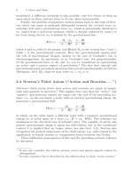
This expression is often complicated, but its meaning can be visualized, as
follows. Consider a stream of particles with current density j
0
per cross-
sectional area flowing towards the target and being scattered by the potential
V. At a large distance beyond the target, a fraction of the particles enters
a counter, where they are recorded. The number of counts in a time Δt is
given by
ΔN =
d
(2)
σ
dΩ

·j
0
· Δt · ΔΩ.
The aperture of the counter corresponds to scattering angles in the interval
(ϑ, ϑ +dϑ), i.e., to the corresponding solid angle element
ΔΩ := 2π sin ϑΔϑ.
The differential scattering cross-section is essentially the missing propor-
tionality factor in the relation
ΔN ∝ j
0
·Δt · ΔΩ,
and (7.1) should only be used for evaluation of this quantity
The description of these relations is supported by Fig. 7.1.
For A/r-potentials the differential cross-section can be evaluated exactly,
with the result
d
(2)
σ
dΩ
=
A
2
16E
2
1
sin
4
ϑ
2
,

which is called the Rutherford scattering cross-section. This result was ob-
tained by Rutherford in Cambridge, U.K., at the beginning of the twentieth
century. At the same time he was able to confirm this formula, motivated by
his ground-breaking scintillation experiments with α-particles. In this way he
discovered that atoms consist of a negatively-charged electron shell with a ra-
dius of the order of 10
−8
cm, and a much smaller, positively-charged nucleus
with a radius of the order of 10
−13
cm. In fact, the differential cross-sections
for atomic nuclei are of the order of 10
−26
cm
2
, i.e., for α-particles the space
between the nuclei is almost empty.
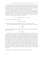
Fig. 7.1. Schematic diagram on differential scattering cross-sections. A particle
enters the diagram from the left on a path parallel to the x-axis at a perpendicular
distance b (the so-called “impact parameter”; here b =0.25). It is then repulsively
scattered by a target at the origin (here the scattering occurs for −20 ≤ x ≤ 20,
where the interaction is felt) and forced to move along the path y(x)=b +0.00025·
(x +20)
2
, until it leaves the diagram asymptotically parallel to the inclined straight
line from the origin (here y =0.016 · x). Finally it enters a counter at a scattering
angle ϑ =arctan0.016, by which the above asymptote is inclined to the x-axis. If
the impact parameter b of the particle is slightly changed (in the (y,z)-plane) to
cover an area element d
(2)

A(b):=dϕ · b · db (where ϕ is the azimuthal angle in
that plane), the counter covers a solid-angle element dΩ(b)=dϕ ·sin ϑ(b) ·dϑ.The
differential cross-section is the ratio
d
(2)
A
dΩ
=
˛
˛
˛
b·db(ϑ)
sin ϑ·dϑ
˛
˛
˛
.
8 Lagrange Formalism I:
Lagrangian and Hamiltonian
In the present context the physical content of the Lagrange formalism (see
below) does not essentially go beyond Newton’s principles; however, mathe-
matically it is much more general and of central importance for theoretical
physics as a whole, not only for theoretical mechanics.
8.1 The Lagrangian Function; Lagrangian
Equations of the Second Kind
Firstly we shall define the notions of “degrees of freedom”, “generalized co-
ordinates”, and the “Lagrangian function” (or simply Lagrangian)assuming
asystemofN particles with 3N Cartesian coordinates x
α
, α =1, ,3N:

a) The number of degrees of freedom f is the dimension of the hypersurface
1
in 3N -dimensional space on which the system moves. This hypersurface
can be fictitious; in particular, it may deform with time. We assume that
we are only dealing with smooth hypersurfaces, such that f only assumes
integral values 1, 2, 3,
b) The generalized coordinates q
1
(t), ,q
f
(t) are smooth functions that
uniquely indicate the position of the system in a time interval Δt around
t; i.e., in this interval x
α
= f
α
(q
1
, ,q
f
,t), for α =1, ,3N. The gen-
eralized coordinates (often they are angular coordinates) are rheonomous,
if at least one of the relations f
α
depends explicitly on t; otherwise they
are called skleronomous.TheLagrangian function L is by definition equal
to the difference (sic) between the kinetic and potential energy of the
system, L = T−V, expressed by q
α
(t), ˙q

α
(t)andt, where it is assumed
that a potential energy exists such that for all α the relation F
α
= −
∂V
∂x
α
holds, and that V can be expressed by the q
i
,fori =1, ,f,andt.
Frictional forces and Lorentz forces (or Coriolis forces, see above) are not al-
lowed with this definition of the Lagrangian function, but the potential energy
may depend explicitly on time. However, one can generalize the definition of
the Langrangian in such a way that Lorentz forces (or Coriolis forces) are
1
For so-called anholonomous constraints (see below), f is the dimension of an
infinitesimal hypersurface element
46 8 Lagrange Formalism I: Lagrangian and Hamiltonian
also included (see below). The fact that the Lagrangian contains the differ-
ence,andnot the sum of the kinetic and potential energies, has a relativistic
origin, as we shall see later.
8.2 An Important Example: The Spherical Pendulum
with Variable Length
These relations are best explained by a simple example. Consider a pendulum
consisting of a weightless thread with a load of mass m at its end. The length
of the thread, l(t), is variable, i.e., an external function. The thread hangs
from the point x
0
= y

0
=0,z
0
= 0, which is fixed in space, and the load
can swing in all directions. In spherical coordinates we thus have (with z
measured as positive downwards): ϑ ∈ [0,π], where ϑ = 0 corresponds to the
position of rest, and ϕ ∈ [0, 2π):
x = l(t) · sin ϑ ·cos ϕ
y = l(t) · sin ϑ · sin ϕ
z = z
0
− l(t) · cos ϑ. (8.1)
The number of degrees of freedom is thus f = 2; the generalized coordinates
are rheonomous, although this is not seen at once, since q
1
:= ϑ and q
2
= ϕ do
not explicitly depend on t, in contrast to the relations between the cartesian
and the generalized coordinates; see (8.1). Furthermore,
V = mgz = mg ·(z
0
− l(t) · cos ϑ) ,
whereas the kinetic energy is more complicated. A long, but elementary cal-
culation yields
T =
m
2

˙x

2
+˙y
2
+˙z
2

≡
m
2

l
2
·

˙
ϑ
2
+sin
2
ϑ ˙ϕ
2

+4l
˙
l sin ϑ cos ϑ
˙
ϑ +
˙
l
2

sin
2
ϑ

.
Apart from an additive constant the Lagrangian L = T−Vis thus:
L(ϑ,
˙
ϑ, ˙ϕ, t)=
m
2

l
2

˙
ϑ
2
+sin
2
ϑ ˙ϕ
2

+4l
˙
l sin ϑ cos ϑ
˙
ϑ
+
˙

l
2
sin
2
ϑ

+ mg ·(l(t) − z
0
) · cos ϑ. (8.2)
(In the expression for the kinetic energy the inertial mass should be used,
and in the expression for the potential energy one should actually use the
gravitational mass; g is the acceleration due to gravity.)
8.3 The Lagrangian Equations of the 2nd Kind 47
8.3 The Lagrangian Equations of the 2nd Kind
These shall now be derived, for simplicity with the special assumption f =1.
Firstly we shall consider an actual orbit q(t), i.e., following the Newtonian
equations transformed from the cartesian coordinate x to the generalized
coordinate q.Attimet
1
this actual orbit passes through an initial point q
1
,
and at t
2
through q
2
. Since Newton’s equation is of second order, i.e., with
two arbitrary constants, this is possible for given q
1
and q

2
.
In the following, the orbit is varied, i.e., a set of so-called virtual orbits,
q
v
(t):=q(t)+ε · δq(t) ,
will be considered, where the real number ε ∈ [−1, 1] is a so-called vari-
ational parameter and δq(t) a fixed, but arbitrary function (continuously
differentiable twice) which vanishes for t = t
1
and t = t
2
.Thus,thevirtual
orbits deviate from the actual orbit, except at the initial point and at the end
point; naturally, the virtual velocities are defined as
˙q
v
(t):= ˙q(t)+ε · δ ˙q(t) , where δ ˙q(t)=
dq(t)
dt
.
Using the Lagrangian function L(q, ˙q,t) one then defines the so-called
action functional
S[q
v
]:=
t
2

t

1
dtL(q
v
, ˙q
v
,t) .
For a given function δq(t) this functional depends on the parameter ε,which
can serve for differentiation. After differentiating with respect to ε one sets
ε = 0. In this way one obtains
dS[q
v
]
dε
|ε=0
=
t
2

t
1
dt

∂L
∂ ˙q
v
δ ˙q(t)+
∂L
∂q
v
δq(t)


. (8.3)
In the first term a partial integration can be performed, so that
dS[q
v
]
dε
|ε=0
=
∂L
∂ ˙q
v
|t
1
δq(t
1
) −
∂L
∂ ˙q
v
|t
2
δq(t
2
)
+
t
2

t

1
dt

−
d
dt
∂L
∂ ˙q
v
+
∂L
∂q
v

δq(t) . (8.4)
In (8.4) the first two terms on the r.h.s. vanish, and since δq(t) is arbitrary,
the action functional S becomes extremal for the actual orbit, q
v
(t) ≡ q(t),
48 8 Lagrange Formalism I: Lagrangian and Hamiltonian
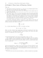
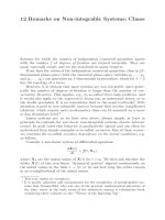
Fig. 8.1. Hamilton’s variational principle. The figure shows the ε-dependent set
of virtual orbits q
v
(t):=t +(t
2
− 1) + ε · sin (t
2
− 1)
3
,forε = −0.6, −0.4, ,0.6

and times t between t
1
= −1andt
2
=1.Theactual orbit, q(t), corresponds to the
central line (ε = 0) and yields an extremum of the action functional. The virtual
orbits can also fan out more broadly from the initial and/or end points than in this
example
iff (i.e., “if, and only if”) the so-called variational derivative
δS
δq
:=

−
d
dt
∂L
∂ ˙q
v
+
∂L
∂q
v

vanishes. An example is shown in Fig. 8.1.
The postulate that S is extremal for the actual orbit is called Hamilton’s
variational principle of least
2
action, and the equations of motion,
d

dt
∂L
∂ ˙q
v
−
∂L
∂q
v
=0,
are called Lagrangian equations of the 2nd kind (called “2nd kind” by some
authors for historical reasons). They are the so-called Euler-Lagrange equa-
tions
3
corresponding to Hamilton’s variational principle. (The more compli-
cated Lagrangian equations of the 1st kind additionally consider constraints
and will be treated in a later section.)
For the special case where
L =
m
2
˙x
2
− V (x) ,
Newton’s equation results. (In fact, the Lagrangian equations of the 2nd kind
can also be obtained from the Newtonian equations by a general coordinate
transformation.) Thus one of the main virtues of the Lagrangian formalism
with respect to the Newtonian equations is that the formalisms are physically
equivalent; but mathematically the Lagrangian formalism has the essential
2
In general, the term “least” is not true and should be replaced by “extremal”.

3
Of course any function F(L), and also any additive modification of L by a total
derivative
df (q(t), ˙q(t),t)
dt
, would lead to the same equations of motion.
8.4 Cyclic Coordinates; Conservation of Generalized Momenta 49
advantage of invariance against general coordinate transformations,whereas
Newton’s equations must be transformed from cartesian coordinates, where
the formulation is rather simple, to the coordinates used, where the formu-
lation at first sight may look complicated and very special.
In any case, the index v, corresponding to virtual, may be omitted, since
finally ε ≡ 0.
For f ≥ 2 the Lagrangian equations of the 2nd kind are, with i =1, ,f:
d
dt
∂L
∂ ˙q
i
=
∂L
∂q
i
. (8.5)
8.4 Cyclic Coordinates; Conservation
of Generalized Momenta; Noether’s Theorem
The quantity
p
i
:=

∂L
∂ ˙q
i
is called the generalized momentum corresponding to q
i
.Oftenp
i
has the
physical dimension of angular momentum, in the case when the corresponding
generalized coordinate is an angle. One also calls the generalized coordinate
cyclic
4
,iff
∂L
∂q
i
=0.
As a consequence, from (8.5), the following theorem
5
is obtained.
If the generalized coordinate q
i
is cyclic, then the related generalized mo-
mentum
p
i
:=
∂L
∂ ˙q
i

is conserved.
As an example we again consider a spherical pendulum (see Sect. 8.2). In
this example, the azimuthal angle ϕ is cyclic even if the length l(t)ofthe
pendulum depends explicitly on time. The corresponding generalized momen-
tum,
p
ϕ
= ml
2
· sin ϑ · ˙ϕ,
is the z-component of the angular momentum, p
i
= L
z
. In the present case,
this is in fact a conserved quantity, as one can also show by elementary argu-
ments, i.e., by the vanishing of the torque D
z
.
4
In general relativity this concept becomes enlarged by the notion of a Killing
vector.
5
The name cyclic coordinate belongs to the canonical jargon of many centuries
and should not be altered.
50 8 Lagrange Formalism I: Lagrangian and Hamiltonian
Compared to the Newtonian equations of motion, the Lagrangian formal-
ism thus:
a) not only has the decisive advantage of optimum simplicity. For suitable
coordinates it is usually quite simple to write down the Lagrangian L of

the system; then the equations of motion result almost instantly;
b) but also one sees almost immediately, because of the cyclic coordinates
mentioned above, which quantities are conserved for the system.
For Kepler-type problems, for example, in planar polar coordinates we di-
rectly obtain the result that
L =
M
2
v
2
s
+
m
2
·

˙r
2
+ r
2
˙ϕ
2

− V (r) .
The center-of-mass coordinates and the azimuthal angle ϕ are therefore
cyclic; thus one has the total linear momentum and the orbital angular mo-
mentum as conserved quantities, and because the Lagrangian does not depend
on t, one additionally has energy conservation, as we will show immediately.
In fact, these are special cases of the basic Noether Theorem, named after
the mathematician Emmy Noether, who was a lecturer at the University of

G¨ottingen, Germany, immediately after World War I. We shall formulate the
theorem without proof (The formulation is consciously quite sloppy):
The three conservation theorems for (i) the total momentum, (ii) the to-
tal angular momentum and (iii) the total mechanical energy correspond (i)
to the homogeneity (= translational invariance) and (ii) the isotropy (rota-
tional invariance) of space and (iii) to the homogeneity with respect to time.
More generally, to any continuous n-fold global symmetry of the system there
correspond n globally conserved quantities and the corresponding so-called
continuity equations, as in theoretical electrodynamics (see Part II).
For the special dynamic conserved quantities, such as the above-mentioned
Runge-Lenz vector, cyclic coordinates do not exist. The fact that these quan-
tities are conserved for the cases considered follows only algebraically using
so-called Poisson brackets, which we shall treat below.
8.5 The Hamiltonian
To treat the conservation of energy, we must enlarge our context somewhat
by introducing the so-called Hamiltonian
H(p
1
, ,p
f
,q
1
, ,q
f
,t) .
This function is a generalized and transformed version of the Lagrangian,
i.e., the Legendre transform of −L, and as mentioned below, it has many
important properties. The Hamiltonian is obtained, as follows:
8.6 The Canonical Equations; Energy Conservation II; Poisson Brackets 51
FirstlywenotethattheLagrangian L depends on the generalized ve-

locities ˙q
i
, the generalized coordinates q
i
and time t. Secondly we form the
function
˜
H(p
1
, ,p
f
, ˙q
1
, , ˙q
f
,q
1
, ,q
f
,t):=
f

i=1
p
i
˙q
i
−L(˙q
1
, , ˙q

1
,q
1
, ,q
f
,t) .
Thirdly we assume that one can eliminate the generalized velocities ˙q
i
by
replacing these quantities by functions of p
i
, q
k
and t with the help of the
equations p
i
≡
∂L
∂ ˙q
i
. This elimination process is almost always possible in
nonrelativistic mechanics; it is a basic prerequisite of the method. After this
replacement one finally obtains
˜
H(p
1
, , ˙q
1
(q
1

, ,p
1
, ,t), ,q
1
, ,t) ≡H(p
1
, ,p
f
,q
1
, ,q
f
,t) .
As already mentioned, the final result, i.e., only after the elimination
process, is called the Hamiltonian of the system. In a subtle way, the Hamil-
tonian is somewhat more general than the Lagrangian, since the variables
p
1
, ,p
f
can be treated as independent and equivalent variables in addition
to the variables q
1
, ,q
f
, whereas in the Lagrangian formalism only the gen-
eralized coordinates q
i
are independent, while the generalized velocities, ˙q
i

,
depend on them
6
. But above all, the Hamiltonian, and not the Lagrangian,
will become the important quantity in the standard formulation of Quantum
Mechanics (see Part III).
8.6 The Canonical Equations;
Energy Conservation II; Poisson Brackets
As a result of the transformation from L to H one obtains:
dH =
f

i=1

dp
i
· ˙q
i
+ p
i
d˙q
i
−
∂L
∂ ˙q
i
d˙q
i
−
∂L

∂q
i
dq
i

−
∂L
∂t
dt.
Here the second and third terms on the r.h.s. compensate for each other, and
from (8.5) the penultimate term can be written as −˙p
i
dq
i
.
Therefore, since dH can also be written as follows:
dH =
f

i=1

dp
i
∂H
∂p
i
+dq
i
∂H
∂q

i

+
∂H
∂t
dt, (8.6)
6
Here we remind ourselves of the natural but somewhat arbitrary definition δ ˙q :=
d(δq)
dt
in the derivation of the principle of least action.
52 8 Lagrange Formalism I: Lagrangian and Hamiltonian
one obtains by comparison of coefficients firstly the remarkable so-called
canonical equations (here not only the signs should be noted):
˙q
i
=+
∂H
∂p
i
, ˙p
i
= −
∂H
∂q
i
,
∂H
∂t
= −

∂L
∂t
. (8.7)
Secondly, the total derivative is
dH
dt
=
f

i=1

˙p
i
∂H
∂p
i
+˙q
i
∂H
∂q
i

+
∂H
∂t
,
and for a general function
F (p
1
(t), ,p

f
(t),q
1
(t), ,q
f
(t),t):
dF
dt
=
f

i=1

˙p
i
∂F
∂p
i
+˙q
i
∂F
∂q
i

+
∂F
∂t
.
Insertion of the canonical equations reduces the previous results to:
dH

dt
=
∂H
∂t
= −
∂L
∂t
and
dF
dt
=
f

i=1

∂H
∂p
i
∂F
∂q
i
−
∂H
∂q
i
∂F
∂p
i

+

∂F
∂t
,
respectively, where we should remember that generally the total and partial
time derivatives are different!
In both cases the energy theorem (actually the theorem of H conservation)
follows:
If L (or H) does not depend explicitly on time (e.g.,
∂H
∂t
≡ 0), then H
is conserved during the motion (i.e.,
dH
dt
≡ 0). Usually, but not always, H
equals the total mechanical energy.
Thus some caution is in order: H is not always identical to the mechanical
energy, and the partial and total time derivatives are also not identical; but
if
L = T−V,
then (if skleronomous generalized coordinates are used) we automatically ob-
tain
H≡T+ V ,
as one can easily derive by a straightforward calculation with the above def-
initions. Here, in the first case, i.e., with L, one should write
T =
mv
2
2
,

whereas in the second case, i.e., with H, one should write
T =
p
2
2m
.