Basic Theoretical Physics: A Concise Overview P9 pdf

11.3 Steiner’s Theorem; Heavy Roller; Physical Pendulum 75
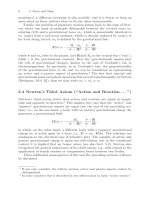
We should mention in this context that modifications of this problem fre-
quently appear in written examination questions, in particular the problem of
the transition from rolling motion down an inclined segment to a subsequent
horizontal motion, i.e., on a horizontal plane segment, and we also mention
the difference between gliding and rolling motions (see below).
As an additional problem we should also mention the physical pendulum,
as opposed to the mathematical pendulum (i.e., a point mass suspended from
a weightless thread or rod), on which we concentrated previously. The physical
pendulum (or compound pendulum) is represented by a rigid body, which is
suspended from an axis around which it can rotate. The center of mass is at
adistances from the axis of rotation, such that
L≡T−V≡
1
2
Θ
˙
ϑ
2
− Mgs·(1 −cos ϑ) .
Here M is the mass of the body, and
Θ := Θ
(s)
+ Ms
2
is the moment of inertia of the rigid body w.r.t. the axis of rotation.
The oscillation eigenfrequency for small-amplitude oscillations is therefore
ω
0
=


g
l
red
,
where the so-called reduced length of the pendulum, l
red
, is obtained from the
following identity:
l
red
=
Θ
Ms
.
At this point we shall mention a remarkable physical “non-event” occur-
ring at the famous Gothic cathedral in Cologne. The towers of the medieval
cathedral were completed in the nineteenth century and political representa-
tives planned to highlight the completion by ringing the so-called Emperor’s
Bell, which was a very large and powerful example of the best technology of
the time. The gigantic bell, suspended from the interior of one of the towers,
was supposed to provide acoustical proof of the inauguration ceremony for
the towers. But at the ceremony, the bell failed to produce a sound, since
the clapper, in spite of heavy activity of the ringing machinery, never actu-
ally struck the outer mantle of the bell
3
. This disastrous misconstruction can
of course be attributed to the fact that the angle of deflection ϑ
1
(t)ofthe
clapper as a function of time was always practically identical with the angle

of deflection of the outer mantle of the bell, i.e., ϑ
2
(t) ≈ ϑ
1
(t) (both angles
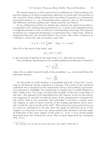
measured from the vertical direction). This is again supported by a diagram
(Fig. 11.1).
3
An exercise can be found on the internet, [2], winter 1992, file 8.
76 11 Rigid Bodies
Fig. 11.1. Schematic diagram for a bell. The diagram shows the mantle of the
bell (the outer double lines, instantaneously swinging to the right) and a clapper
(instantaneously swinging to the left). It is obvious from this sketch that there
are two characteristic angles for the bell, the first one characterizing the deviation
of the center of mass (without clapper) from the vertical, the second one for the
clapper itself.
The reason for the failure, which is often used as a typical examination
question on the so-called double compound pendulum, is that the geometrical
and material parameters of the bell were such that
l
red|{bell with fastened clapper}
≈ l
red|{clapper alone}
.
Another remarkable example is the reversion pendulum.Ifwestartfrom
the above-mentioned equation for the reduced length of the pendulum, inser-
tion of the relation
Θ
!
= Θ

(s)
+ Ms
2
gives l
red
(s)
!
=
Θ
(s)
Ms
+ s.
This yields a quadratic equation with two solutions satisfying
s
1
+ s
2
= l
red
.
For a given system, i.e., with given center of mass, we thus obtain two solu-
tions, with
s
2
= l
red
− s
1
.
If we let the pendulum oscillate about the first axis, i.e., corresponding to

the first solution s
1
, then, for small oscillation amplitudes we obtain the
oscillation eigenfrequency
ω
0
=

g
l
red
.
If, subsequently, after reversion, we let the pendulum oscillate about the par-
allel second axis, i.e., corresponding to s
2
, then we obtain the same frequency.
11.4 Inertia Ellipsoids; Poinsot Construction 77
11.4 Inertia Ellipsoids; Poinsot Construction
The positive-definite quadratic form
2T
rot
=
3

i,k=1
θ
i,k
ω
i
ω

k
describes an ellipsoid within the space R
3
(ω), the so-called inertia ellipsoid.
This ellipsoid can be diagonalized by a suitable rotation, and has the
normal form
2T
rot
=
3

α=1
Θ
α
· ω
2
α
,
with so-called principal moments of inertia Θ
α
and corresponding principal
axes of lengths
a
α
=

2T
rot
Θ
α

.
(See Fig. 11.2.)
Every rigid body, however arbitrarily complex, possesses such an inertia
ellipsoid. This is a smooth fictitious body, in general possessing three principal
axes of different length, and where the directions of the principal axes are not
easily determined. However, if the body possesses a (discrete!) n-fold axis of
rotation
4
,withn ≥ 3, then the inertia ellipsoid is an ellipsoid of (continuous!)
revolution around the symmetry axis.
As a practical consequence, e.g., for a three-dimensional system with
a square base, this implies the following property. If the system is rotated
about an arbitrary axis lying in the square, then the rotational energy of
the system does not depend on the direction of the rotation vector ω, e.g.,
whether it is parallel to one of the edges or parallel to one of the diagonals;
it depends only on the magnitude of the rotational velocity.
The angular momentum L is calculated by forming the gradient (w.r.t.
ω)ofT
rot
(ω). Thus
L(ω) = grad
ω
T
rot
(ω) , i.e., L
α
=
∂T
rot
∂ω

α
= Θ
α
ω
α
.
Since the gradient vector is perpendicular to the tangent plane of T
rot
(ω),
one thus obtains the so-called Poinsot construction:
For given vector of rotation the angular momentum L(ω) is by construc-
tion perpendicular to the tangential plane of the inertial ellipsoid T
rot
(ω)=
constant corresponding to the considered value of ω. This can be seen in
Fig. 11.2.
4
This means that the mass distribution of the system is invariant under rotations
about the symmetry axis by the angle 2π/n.
78 11 Rigid Bodies
Fig. 11.2. Inertia ellipsoid and Poinsot con-
struction. For the typical values a := 2 and
b := 1, a (ω
x
,ω
y
)-section of an inertia ellip-
soid
ω
2

1
Θ
1
+ +
ω
2
3
Θ
3
=2· T
rot
(with, e.g.,
a
2
≡
2·T
rot
Θ
1
) and an initial straight line
(here diagonal) through the origin is plot-
ted as a function of ω
x
. The second (exter-
nal) straight line is perpendicular to the tan-
gential plane of the first line, i.e., it has the
direction of the angular momentum L.This
is the so-called Poinsot construction
One can also define another ellipsoid, which is related to the inertia el-
lipsoid, but which is complementary or dual to it, viz its Legendre transform.

The transformed ellipsoid or so-called Binet ellipsoid is not defined in the
space R
3
(ω), but in the dual space R
3
(L)bytherelation
2T
rot
=
3

α=1
L
2
α
Θ
α
.
Instead of the angular velocity ω,theangular momentum L is now central.
In fact, L and ω are not parallel to each other unless ω has the direction of
a principal axis of the inertia ellipsoid.
We shall return to this point in Part II, while discussing crystal optics,
when the difference between the directions of the electric vectors E and D
is under debate.
11.5 The Spinning Top I: Torque-free Top
A spinning top is by definition a rigid body supported at a canonical reference
point r
0
(see above), where in general v
0

= 0. For example, r
0
is the point
of rotation of the rigid body on a flat table. In this case, the gravitational
forces, virtually concentrated at the center of mass, produce the following
torques w.r.t. the point of rotation of the top on the table:
D
r
0
=(R
s
− r
0
) ×(−Mgˆz) .
A torque-free top is by definition supported at its center of mass; there-
fore no gravitational torque does any work on the top. The total angular
momentum L is thus conserved, as long as external torques are not applied,
which is assumed. Hence the motion of the torque-free top can be described as
a “rolling of the inertia ellipsoid along the Poinsot plane”, see above. In this
way, ω-lines are generated on the surface of the inertia ellipsoid as described
in the following section.
11.6 Euler’s Equations of Motion and the Stability Problem 79
11.6 Euler’s Equations of Motion
and the Stability Problem
We now wish to describe the stability of the orbits of a torque-free top.There-
fore we consider as perturbations only very weak transient torques. Firstly,
we have
ω(t)=
3


α=1
ω
α
(t)e
α
(t)andL =
3

α=1
L
α
(t)e
α
(t) .
Here the (time-dependent) unit vectors e
α
(t) describe the motion of the prin-
cipal axes of the (moving) inertia ellipsoid; ω
α
(t)andL
α
(t) are therefore
co-moving cartesian coefficients of the respective vectors ω and L; i.e., the
co-moving cartesian axes e
α
(t), for α =1, 2, 3, are moving with the rigid
body, to which they are fixed and they depend on t,whereastheaxese
j
,for
j = x, y, z, are fixed in space and do not depend on t:

L
α
(t) ≡ L
α
(t)
|co−moving
,
ω
α
(t) ≡ ω
α
(t)
|co−moving
.
But
d
dt
e
α
= ω × e
α
;
hence
d
dt
L =
3

α=1


dL
α
dt

|co−moving
e
α
(t)+ω × L = δD(t) , (11.6)
where the perturbation on the right describes the transient torque.
We also have
d
dt
ω =
3

α=1

dω
α
dt

|co−moving
e
α
(t) .
Hence in the co-moving frame of the rigid body:

dL
α
dt


+ ω
β
L
γ
− ω
γ
L
β
= δD
α
etc., and with L
α
= Θ
α
ω
α
we obtain the (non-linear) Euler equations for the
calculation of the orbits ω(t) on the surface of the inertia ellipsoid:
Θ
α
·

dω
α
dt

+ ω
β
ω

γ
·(Θ
γ
− Θ
β
)=δD
α
(t) ,
Θ
β
·

dω
β
dt

+ ω
γ
ω
α
· (Θ
α
− Θ
γ
)=δD
β
(t) ,
80 11 Rigid Bodies
Θ
γ

·

dω
γ
dt

+ ω
α
ω
β
·(Θ
β
− Θ
α
)=δD
γ
(t) . (11.7)
Let us now consider the case of an ellipsoid with three different principal
axes and assume without lack of generality that
Θ
α
<Θ
β
<Θ
γ
.
In (11.7), of the three prefactors
∝ ω
β
ω

γ
, ∝ ω
γ
ω
α
and ∝ ω
α
ω
β
the first and third are positive, while only the second (corresponding to the
so-called middle axis) is negative. As a consequence, small transient perturba-
tions δD
α
and δD
γ
lead to elliptical motions around the respective principal
axis, i.e.,
∝

ε
β
ω
2
β
+ ε
γ
ω
2
γ


and ∝

ε
α
ω
2
α
+ ε
β
ω
2
β

,
whereas perturbations corresponding to δD
β
may have fatal effects, since in
the vicinity of the second axis the ω-lines are hyperbolas,
∝

ε
α
ω
2
α
− ε
γ
ω
2
γ


,
i.e., along one diagonal axis they are attracted, but along the other diagonal
axis there is repulsion, and the orbit runs far away from the axis where it
started.
The appearance of hyperbolic fixed points is typical for the transition to
chaos, which is dicussed below.
Motion about the middle axis is thus unstable.
This statement can be shown to be plausible by plotting the orbits in
the frame of the rotating body for infinitesimally small perturbations, δD →
0, The lines obtained in this way on the surface of the inertia ellipsoid by
integration of the three coupled equations (11.7) describe the rolling motion
of the inertia ellipsoid on the Poinsot plane. Representations of these lines
can be found in almost all relevant textbooks.
Another definition for the ω-lines on the inertia ellipsoid is obtained as
follows: they are obtained by cutting the inertia ellipsoid
3

α=1
Θ
α
ω
2
i
=2T
rot
= constant

.
with the so-called L

2
or swing ellipsoid , i.e., the set
3

α=1
Θ
2
α
ω
2
i
= L
2
= constant

.
We intentionally omit a proof of this property, which can be found in many
textbooks.
11.7 The Three Euler Angles ϕ, ϑ and ψ; the Cardani Suspension 81
To calculate the Hamiltonian it is not sufficient to know
d
dt
ω
α|co−moving
.
Therefore we proceed to the next section.
11.7 The Three Euler Angles ϕ, ϑ and ψ;
the Cardani Suspension
Apart from the location of its center of mass, the position of a rigid body
is characterized by the location in space of two orthogonal axes fixed within

the body : e
3
and e
1
. For example, at t = 0 we may assume
e
3
≡ ˆz and e
1
(without prime) ≡ ˆx .
For t>0 these vectors are moved to new directions:
e
3
(0) → e
3
(t)(≡ e
3
)ande
1
→ e

1
(now with prime) .
This occurs by a rotation D
R
, which corresponds to the three Euler angles
ϕ, χ and ψ, as follows (the description is now general):
a) Firstly, the rigid body is rotated about the z-axis(whichisfixedinspace)
by an angle of rotation ϕ, in such a way that the particular axis of the
rigid body corresponding to the ˆx direction is moved to a so-called node

direction e
1
.
b) Next, the particular axis, which originally (e.g., for t =0)pointsinthe
ˆz-direction, is tilted around the nodal axis e
1
in the e
3
direction by an
angle ϑ = arccos(ˆz ·e
3
).
c) Finally, a rotation by an angle ψ around the e
3
axis follows in such a way
that the nodal direction, e
1
, is rotated into the final direction e

1
.
As a consequence we obtain
D
R
≡D
3)
e
3
(ψ) ·D
2)

e
1
(ϑ) ·D
1)
ˆz
(ϕ) ,
where one reads from right to left, and the correct order is important, since fi-
nite rotations do not commute (only infinitesimal rotations would commute).
A technical realization of the Euler angles is the well-known Cardani sus-
pension , a construction with a sequence of three intertwined rotation axes
in independent axle bearings (see the following text). In particular this is
a realization of the relation
ω =
˙
ψe
3
+
˙
ϑe
1
+˙ϕˆz ,
which corresponds to the special case of infinitesimal rotations; this relation
will be used below.
82 11 Rigid Bodies
In the following we shall add a verbal description of the Cardani suspen-
sion, which (as will be seen) corresponds perfectly to the Euler angles.
The lower end of a dissipationless vertical rotation axis, 1 ( ˆ= ± ˆz,cor-
responding to the rotation angle ϕ), branches into two axle bearings, also
dissipationless, supporting a horizontal rotation axis, 2 (= ±e
1

), with corre-
sponding rotation angle ϑ around this axis.
This horizontal rotation axis corresponds in fact to the above-mentioned
nodal line; in the middle, this axis branches again (for ϑ = 0: upwards and
downwards) into dissipationless axle bearings, which support a third rotation
axis, 3, related to the direction e
3
(i.e., the figure axis), with rotation angle
ψ. For finite ϑ, this third axis is tilted with respect to the vertical plane
through ˆz and e
1
. The actual top is attached to this third axis.
Thus, as mentioned, for the so-called symmetrical top, i.e., where one is
dealing with an inertia ellipsoid with rotational symmetry, e.g.,
Θ
1
≡ Θ
2
,
the (innermost) third axis of the Cardani suspension corresponds to the so-
called figure axis of the top.
The reader is strongly recommended to try to transfer this verbal descrip-
tion into a corresponding sketch! The wit of the Cardani suspension is that
the vertical axis 1 branches to form the axle bearings for the horizontal nodal
axis, 2, and this axis provides the axle bearings for the figure axis 3.
To aid the individual imagination we present our own sketch in Fig. 11.3.
TheimportanceoftheEuler angles goes far beyond theoretical mechanics
as demonstrated by the technical importance of the Cardani suspension.
Fig. 11.3. The figure illustrates a so-called Cardani sus-
pension, which is a construction involving three different

axes of rotation with axle bearings, corresponding to the
Euler angles ϕ, ϑ and ψ
11.8 The Spinning Top II: Heavy Symmetric Top 83
11.8 The Spinning Top II: Heavy Symmetric Top
The “heavy symmetric top” is called heavy, because it is not supported at
the center of mass, so that gravitational forces now exert a torque, and it is
called symmetric, because it is assumed, e.g., that
Θ
1
≡ Θ
2
(= Θ
3
) .
The axis corresponding to the vector e
3
is called the figure axis. Additionally
one uses the abbreviations
Θ
⊥
:= Θ
1
≡ Θ
2
and Θ
||
:= Θ
3
.
Let us calculate the Lagrangian

L(ϕ, ϑ, ψ, ˙ϕ,
˙
ϑ,
˙
ψ) .
Even before performing the calculation we can expect that ψ and ϕ are cyclic
coordinates, i.e., that
∂L
∂ϕ
=
∂L
∂ψ
=0,
such that the corresponding generalized momenta
p
ϕ
:=
∂L
∂ ˙ϕ
and p
ψ
:=
∂L
∂
˙
ψ
are conserved quantities.
Firstly, we express the kinetic energy
T
rot

:=
1
2
·

Θ
⊥
·

ω
2
1
+ ω
2
2

+ Θ
||
ω
2
3

in terms of the Euler angles by
ω =
˙
ψe
3
+
˙
ϑe

1
+˙ϕˆz .
Scalar multiplication with e
3
, e
1
and e
2
yields the result
5
:
ω
3
=
˙
ψ +˙ϕ ·cos ϑ,
ω
1
=
˙
ϑ and
ω
2
=˙ϕ · sin ϑ.
As a consequence, we have
T
rot
=
Θ
⊥

2
·

˙
ϑ
2
+sin
2
ϑ ˙ϕ
2

+
Θ
||
2
·

˙
ψ +˙ϕ cos ϑ

2
. (11.8)
5
because e
3
, ˆz and e
2
are co-planar, such that e
3
· ˆz =cosϑ and e

2
· ˆz =sinϑ.
84 11 Rigid Bodies
Additionally we have the potential energy
V = Mgs· cos ϑ, where s ·cos ϑ
is the z-component of the vector (R
s
− r
0
). The Lagrangian is
L =T
rot
−V.
Obviously ψ and ϕ are cyclic, and the above-mentioned generalized momenta
are conserved, viz the following two components of the angular momentum L:
p
ψ
=
∂T
rot
∂
˙
ψ
= Θ
||
· (
˙
ψ +˙ϕ cos ϑ)=Θ
||
ω

3
≡ L
3
≡ L(t) ·e
3
(t) , and
p
ϕ
=
∂T
rot
∂ ˙ϕ
= Θ
⊥
·sin
2
ϑ ˙ϕ + Θ
||
·(
˙
ψ +˙ϕ cos ϑ)cosϑ
= Θ
2
ω
2
sin ϑ + Θω
3
cos ϑ
= L
2

sin ϑ + L
3
cos ϑ ≡ L
z
≡ L(t) · ˆz .
The symmetric heavy top thus has exactly as many independent
6
con-
served quantities as there are degrees of freedom. The number of degrees of
freedom is f = 3, corresponding to the three Euler angles,andthethree
independent conserved quantities are:
a) The conservation law for the (co-moving!) component L
3
of the angu-
lar momentum, i.e., the projection onto the (moving!) figure axis.(This
conservation law is remarkable, in that the figure axis itself performs
a complicated motion. On the one hand the figure axis precesses around
the (fixed) z-axis; on the other hand, it simultaneously performs so-called
nutations, i.e., the polar angle ϑ(t) does not remain constant during the
precession, but performs a more-or-less rapid periodic motion between
two extreme values.)
For the asymmetric heavy top this conservation law would not be true.
b) The component L
z
of the angular momentum (fixed in space!).
c) As a third conservation law we have, of course, conservation of energy,
since on the one hand the Lagrangian L does not depend explicitly on
time, while on the other hand we have used skleronomous coordinates,
i.e., the relation between the Euler angles and the cartesian coordinates
x, y and z does not explicitly depend on time.

6
Two dependent conserved quantities are e.g., the Hamiltonian H of a conservative
system and any function F (H).