Basic Theoretical Physics: A Concise Overview P12 pdf

16 Introduction and Mathematical
Preliminaries to Part II
The theory of electrodynamics provides the foundations for most of our
present-day way of life, e.g., electricity, radio and television, computers, radar,
mobile phone, etc.; Maxwell’s theory lies at the heart of these technologies,
and his equations at the heart of the theory.
Exercises relating to this part of the book (originally in German, but now
with English translations) can be found on the internet, [2].
Several introductory textbooks on theoretical electrodynamics and as-
pects of optics can be recommended, in particular “Theoretical Electrody-
namics” by Thorsten Fliessbach (taken from a comprehensive series of text-
books on theoretical physics). However, this author, like many others, exclu-
sively uses the Gaussian (or cgs) system of units (see below). Another book
of lasting value is the text by Bleaney and Bleaney, [10], using mksA units,
and containing an appendix on how to convert from one system to the other.
Of similar value is also the 3rd edition of the book by Jackson, [11].
16.1 Different Systems of Units in Electromagnetism
In our treatment of electrodynamics we shall adopt the international sys-
tem (SI) throughout. SI units are essentially the same as in the older mksA
system, in that length is measured in metres, mass in kilograms, time in
seconds and electric current in amp`eres. However other systems of units,
in particular the centimetre-gram-second (cgs) (or Gaussian) system, are
also in common use. Of course, an mks system (without the “A”) would
be essentially the same as the cgs system, since 1 m = 100 cm and
1 kg = 1000g. In SI, the fourth base quantity, the unit of current, amp`ere
(A), is now defined via the force between two wires carrying a current. The
unit of charge, coulomb (C), is a derived quantity, related to the amp`ere
by the identity 1 C = 1 A.s. (The coulomb was originally defined via the
amount of charge collected in 1 s by an electrode of a certain electrolyte
system.) For theoretical purposes it might have been more appropriate to
adopt the elementary charge |e| =1.602 · 10

−19
C as the basic unit of
charge; however, this choice would be too inconvenient for most practical
purposes.
110 16 Introduction and Mathematical Preliminaries to Part II
The word “electricity” originates from the ancient Greek word ελεκτoν,
meaning “amber”, and refers to the phenomenon of frictional or static elec-
tricity. It was well known in ancient times that amber can be given an electric
charge by rubbing it, but it was not until the eighteenth century that the law
of force between two electric charges was derived quantitatively: Coulomb’s
law
1
states that two infinitesimally small charged bodies exert a force on each
other (along the line joining them), which is proportional to the product of
the charges and inversely proportional to the square of the separation. In SI
Coulomb’s law is written
F
1←2
=
q
1
q
2
4πε
0
r
2
1,2
e
1←2

, (16.1)
where the unit vector e
1←2
describes the direction of the line joining the
charges,
e
1←2
:= (r
1
− r
2
)/|r
1
− r
2
| , while r
1,2
:= |r
1
− r
2
|
is the distance between the charges.
According to (16.1), ε
0
,thepermittivity of free space,hasthephysical
dimensions of charge
2
/(length
2

·force).
In the cgs system, which was in general use before the mksA system had
been introduced
2
,thequantity4πε
0
in Coulomb’s law (16.1) does not appear
at all, and one simply writes
F
1←2
=
q

1
q

2
r
2
1,2
e
1←2
. (16.2)
Hence, the following expression shows how charges in cgs units (primed)
appear in equivalent equations in mksA or SI (unprimed) (1a):
q

⇔
q
√

4πε
0
,
i.e., both charges differ only by a factor, which has, however, a physical
dimension.
(Also electric currents, dipoles, etc., are transformed in a similar way to
electric charges.) For other electrical quantities appearing below, the relations
are different, e.g., (2a):
E

⇔ E ·
√
4πε
0
(i.e., q

· E

= qE(≡ F )); and, (3a):
D

⇔ D ·

4π
ε
0
1
Charles Augustin de Coulomb, 1785.
2
Gauß was in fact an astronomer at the university of G¨ottingen, although perhaps

most famous as a mathematician.
16.1 Different Systems of Units in Electromagnetism 111
(where in vacuo D := ε
0
E, but D

:= E

). For the magnetic quantities we
have analogously, (1b):
m

⇔
m
√
4πμ
0
;
(2b):
H

⇔ H ·

4πμ
0
;
(3b):
B

⇔ B ·


4π
μ
0
, where μ
0
:=
1
ε
0
c
2
,
with the light velocity (in vacuo) c; m is the magnetic moment, while H and
B are magnetic field and magnetic induction, respectively.
Equations (1a) to (3b) give the complete set of transformations between
(unprimed) mksA quantities and the corresponding (primed) cgs quantities.
These transformations are also valid in polarized matter.
Since ε
0
does not appear in the cgs system – although this contains a com-
plete description of electrodynamics – it should not have a fundamental sig-
nificance per se in SI. However, Maxwell’s theory (see later) shows that ε
0
is
unambiguously related to μ
0
, the equivalent quantity for magnetic behavior,
via c, the velocity of light (i.e., electromagnetic waves) in vacuo, viz
ε

0
μ
0
≡
1
c
2
.
Now since c has been measured to have the (approximate) value 2.998 ·
10
8
m/s, while μ
0
,thevacuum permeability, has been defined by international
convention
3
to have the exact value
μ
0
≡ 4π · 10
−7
Vs/(Am) ,
4
then ε
0
is essentially determined in terms of the velocity of light; ε
0
(≡
1/(μ
0

· c
2
)) has the (approximate) value 8.854 · 10
−12
As/(Vm).
In SI, Maxwell’s equations (in vacuo)are:
divE = /ε
0
, divB =0, curlE = −
∂B
∂t
, curlB = μ
0
j +
1
c
2
∂E
∂t
. (16.3)
These equations will be discussed in detail in the following chapters.
The equivalent equations in a Gaussian system are (where we write the
quantities with a prime):
divE

=4π

, divB

=0, curlE


= −
∂B

∂ct
, curlB

=
4π
c
j

+
∂E

∂ct
. (16.4)
3
essentially a political rather than a fundamentally scientific decision!
4
This implies that B

=10
4
Gauss corresponds exactly to B =1Tesla.
112 16 Introduction and Mathematical Preliminaries to Part II
One should note the different powers of c in the last terms of (16.3) and
(16.4).
Another example illustrating the differences between the two equivalent
measuring systems is the equation for the force exerted on a charged particle

moving with velocity v in an electromagnetic field, the so-called Lorentz force:
In SI this is given by
F = q · (E + v × B) , (16.5)
whereas in a Gaussian system the expression is written
F = q

·

E

+
v
c
× B


We note that all relationships between electromagnetic quantities can be
expressed equally logically by the above transformations in either an SI system
(“SI units”) or a Gaussian system (“Gaussian units”). However, one should
never naively mix equations from different systems.
16.2 Mathematical Preliminaries I: Point Charges
and Dirac’s δ Function
A slightly smeared point charge of strength q at a position r

can be described
by a charge density

ε
(r)=q · δ
ε

(r − r

) , where δ
ε
is a suitable rounded function (see Fig. 16.1) and ε is a corresponding smear-
ing parameter. For all positive values of ε the integral

d
3
rδ
ε
(r − r

)
!
=1,
although at the same time the limit lim
ε→0
δ
ε
(r) shall be zero for all r =0.It
can be shown that this is possible, e.g., with a Gaussian function
δ
ε
(r − r

)=
exp

−

|r−r

|
2ε
2

(2πε
2
)
3/2
(in three dimensions, d =3).
16.2 Mathematical Preliminaries I: Point Charges and Dirac’s δ Function 113
The functions δ
ε
(r −r

) are well-behaved for ε = 0 and only become very
“spiky” for ε → 0
5
, i.e.,
δ(r − r

) := lim
ε→0
δ
ε
(r −r

) ,
where the limit should always be performed in front of the integral, as in the

following equations (16.6) and (16.7).
For example, let f(r) be a test function, which is differentiable infinitely
often and nonzero only on a compact set ∈R
3
; for all these f we have

d
3
r

δ(r

− r) · f(r

) := lim
ε→0

d
3
r

δ
ε
(r

− r) ·f(r

) ≡ f(r) . (16.6)
In the “weak topology” case considered here, the δ-function can be dif-
ferentiated arbitrarily often

6
: Since the test function f (r) is (continuously)
differentiable with respect to the variable x, one obtains for all f by a partial
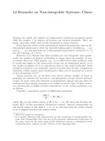
Fig. 16.1. Gaussian curves as an approximation for Dirac’s δ-function. Here we
consider one-dimensional Gaussian curves (for y between 0 and 2)
δ
ε
(x):=(2πε
2
)
−0.5
exp(−x
2
/(2ε
2
)) plotted versus x (between −1and1)within-
creasing sharpness, ε =0.2, 0.1and0.05, which serve as approximations of Dirac’s
δ-function for d = 1; this function is obtained in the limit ε → 0, where the limit is
performed in front of an integral of the kind mentioned in the text
5
Dirac’s δ-function is sometimes referred to as a “spike function”; in particular,
the function δ
ε
(x) (for d=1) is often defined via the limit ε → 0ofδ
ε
(x)=1/ε
for |x|≤ε/2, otherwise = 0. This is convenient in view of the normalization;
however, because of (16.7) we recommend modifying these functions slightly by
smearing them somewhat, i.e., at the sharp edges they should be made differen-
tiable infinitely often.

6
This may be somewhat surprising, if one abides by the simple proposition of an
infinitely high spike function corresponding to the popular definition δ(x) ≡ 0
for x = 0, but δ(0) is so large that
R
dxδ(x) = 1, i.e., if one does not keep in
mind the smooth definition of the approximants δ
ε
(x).
114 16 Introduction and Mathematical Preliminaries to Part II
integration:

d
3
r

∂
∂x

δ(r

− r) · f(r

) := lim
ε→0

d
3
r


∂
∂x

δ
ε
(r

− r) · f(r

)
≡ (−1)
∂
∂x
f(r) . (16.7)
To summarize:apointchargeofstrengthq, located at r

, can be formally
described by a charge density given by:
(r)=q ·δ(r − r

) . (16.8)
16.3 Mathematical preliminaries II: Vector Analysis
and the Integral Theorems of Gauss and Stokes
In this section we shall remind ourselves of a number of important mathe-
matical operators and theorems used in electrodynamics. Firstly, the vector
operator nabla
∇ :=

∂
∂x

,
∂
∂y
,
∂
∂z

(16.9)
is used to express certain important operations, as follows:
a) The gradient of a scalar function f(r) is a vector field defined by
gradf(r):=∇f(r)=(∂
x
f(r),∂
y
f(r),∂
z
f(r)) , (16.10)
where we have used the short-hand notation
∂
j
:=
∂
∂x
j
.
This vector, gradf(r), is perpendicular to the surfaces of constant value
of the function f (r) and corresponds to the steepest increase of f (r). In
electrodynamics it appears in the law relating the electrostatic field E(r)
to its potential φ(r)(E = −gradφ). The minus sign is mainly a matter of
convention, as with the force F and the potential energy V in mechanics.)

b) The divergence (or source density)ofv(r) is a scalar quantity defined
as
divv(r):=∇·v(r)=∂
x
v
x
+ ∂
y
v
y
+ ∂
z
v
z
. (16.11)
It is thus formed from v(r) by differentiation plus summation
7
.Thefact
that this quantity has the meaning of a source density follows from the
integral theorem of Gauss (see below).
7
One should not forget to write the “dot” for the scalar multiplication (also called
“dot product”) of the vectors v
1
and v
2
, since for example c := ∇v (i.e., without
·), would not be a scalar quantity, but could be a second-order tensor, with
theninecomponentsc
i,k

=
∂v
k
∂x
i
. However, one should be aware that one can
encounter different conventions concerning the presence or absence of the dot in
a scalar product.
16.3 Mathematical Preliminaries II: Vector Analysis 115
c) The curl (or circulation density) of a vector field v(r) is a vector quantity,
defined as
curlv(r):=∇×v(r)=[∂
y
v
z
−∂
z
v
y
,∂
z
v
x
−∂
x
v
z
,∂
x
v

y
−∂
y
v
x
] . (16.12)
(The term rotv is also used instead of curlv and the ∧ symbol in-
stead of ×.) Additionally, curl can be conveniently expressed by means
of the antisymmetric unit tensor and Einstein’s summation convention
8
,
(curlv)
i
= e
ijk
∂
j
v
k
).
The fact that this quantity has the meaning of a circulation density follows
from the integral theorem of Stokes, which we shall describe below.
Having introduced the operators grad, div and curl, we are now in a po-
sition to describe the integral theorems of Gauss and Stokes.
a) Gauss’s theorem
Let V (volume) be a sufficiently smooth oriented
9
3d-manifold with closed
boundary ∂V and (outer) normal n(r). Moreover, let a vector field v(r)
be continuous on ∂V and continuously differentiable in the interior of V

10
.
Then Gauss’s theorem states that


∂V
v(r) · n(r)d
2
A =

V
divv(r)d
3
V. (16.13)
Here d
2
A is the area of an infinitesimal surface element of ∂V and d
3
V is
the volume of an infinitesimal volume element of V . The integral on the
l.h.s. of equation (16.13) is the “flux” of v out of V through the surface
∂V . The integrand divv(r) of the volume integral on the r.h.s. is the
“source density” of the vector field v(r).
In order to make it more obvious that the l.h.s. of (16.13) represents
a flux integral, consider the following: If the two-dimensional surface ∂V
is defined by the parametrization
∂V := {r|r =(x(u, v),y(u, v),z(u, v))} , (16.14)
with (u, v) ∈ G(u, v), one then has on the r.h.s. of the following equation
an explicit double-integral, viz



∂V
v(r) · n(r)d
2
A ≡

G(u,v)
v(r(u, v)) ·

∂r
∂u
×
∂r
∂v

dudv. (16.15)
8
Indices appearing two times (here j and k) are summed over.
9
“Inner” and “outer” normal direction can be globally distinguished.
10
These prerequisites for Gauss’s integral theorem (and similar prerequites for
Stokes’s theorem) can of course be weakened.
116 16 Introduction and Mathematical Preliminaries to Part II
b) Stokes’s theorem
Let Γ be a closed curve with orientation, and let F be a sufficiently
smooth 2d-manifold with (outer) normal n(r) inserted
11
into Γ , i.e., Γ ≡
∂F.Moreover,letv(r) be a vector field, which is continuous on ∂F and

continuously differentiable in the interior of F. The theorem of Stokes
then states that

∂F
v(r) · dr =

F
curlv(r) · n(r)d
2
A. (16.16)
The line integral on the l.h.s. of this equation defines the “circulation” of v
along the closed curve Γ = ∂F. According to Stokes’s theorem this quan-
tity is expressed by a 2d-surface integral over the quantity curlv·n. Hence
it is natural to define curlv as the (vectorial) circulation density of v(r).
Detailed proofs of these integral theorems can be found in many mathe-
matical textbooks. Here, as an example, we only consider Stokes’s theorem,
stressing that the surface F is not necessarily planar. But we assume that it
can be triangulated, e.g., paved with infinitesimal triangles or rectangles, in
each of which “virtual circulating currents” flow, corresponding to the chosen
orientation, such that in the interior of F the edges of the triangles or rect-
angles run pairwise in opposite directions, see Fig. 16.2. It is thus sufficient to
prove the theorem for infinitesimal rectangles R. Without lack of generality, R
is assumed to be located in the (x,y)-plane; the four vertices are assumed to be
P
1
=(−Δx/2, −Δy/2) (i.e., lower left) ,
P
2
=(+Δx/2, −Δy/2) (i.e., lower right) ,
P

3
=(+Δx/2, +Δy/2) (i.e., upper right) and
P
4
=(−Δx/2, +Δy/2) (i.e., upper left) .
Therefore we have

∂R
v ·dr
∼
=
[v
x
(0, −Δy/2) −v
x
(0, +Δy/2)]Δx
+[v
y
(+Δx/2, 0) −v
y
(−Δx/2), 0)] Δy
∼
=

−
∂v
x
∂y
+
∂v

y
∂x

ΔxΔy
=

R
curlv · nd
2
A. (16.17)
11
To aid understanding, it is recommended that the reader produces his or her
own diagram of the situation. Here we are somewhat unconventional: usually
one starts with a fixed F , setting ∂F = Γ ; however we prefer to start with Γ ,
since the freedom to choose F ,forfixedΓ (→ ∂F), is the geometrical reason for
the freedom of gauge transformations, see below.
16.3 Mathematical Preliminaries II: Vector Analysis 117
Fig. 16.2. Stokes’s theorem: triangulating
a 2d-surface in space. As an example, the
surface z = xy
2
is triangulated (i.e., paved)
by a grid of small squares. If all the squares
are oriented in the same way as the out-
ermost boundary line, then in the interior
ofthesurfacethelineintegralsareper-
formed in a pairwise manner in the oppo-
site sense, such that they compensate each
other, leaving only the outermost boundary
lines. As a consequence, if the integral theo-

rem of Stokes applies for the small squares,
then it also applies for a general surface
With n =(0, 0, 1) and d
2
A =dxdy this provides the statement of the
theorem.
12
12
Because of the greater suggestive power, in equations (16.17) we have used
H
∂R
instead of
R
∂R
.
17 Electrostatics and Magnetostatics
17.1 Electrostatic Fields in Vacuo
17.1.1 Coulomb’s Law and the Principle of Superposition
The force on an electric point charge of strength q at the position r

in an
electric field E(r

) (passive charge, local action) is given by
F (r

)=qE(r

) . (17.1)
This expression defines the electric field E via the force acting locally on the

passive charge q. However, the charge itself actively generates a field E(r)at
a distant position r (active charge, action at a distance) given by:
E(r)=
q · (r − r

)
4πε
0
|r − r

|
3
. (17.2)
Thefactthattheactive and passive charges are the same (apart from
a multiplicative constant of nature such as c, which can be simply replaced
by 1 without restriction) is not self-evident, but is essentially equivalent to
Newton’s third axiom. One consequence of this is the absence of torques in
connection with Coulomb’s law for the force between two point charges:
F
1,2
=
q
1
q
2
·(r
1
− r
2
)

4πε
0
|r
1
− r
2
|
3
(= −F
2,1
) . (17.3)
Similar considerations apply to gravitational forces; in fact, “gravitational
mass” could also be termed “gravitational charge”, although an essential
difference from electric charges is that inter alia electric charges can either
have a positive or a negative sign, so that the force between two electric
charges q
1
and q
2
can be repulsive or attractive according to the sign of
q
1
q
2
, whereas the gravitational force is always attractive, since “gravitational
charges” always have the same sign, while the gravitational constant leads to
attraction (see (17.4)).
Certainly, however, Newton’s law of gravitation,
(F
gravitation

)
1,2
= −γ
m
1
m
2
·(r
1
− r
2
)
|r
1
− r
2
|
3
, (17.4)