Networking Theory and Fundamentals - Lectures 9 & 10 pps
Bạn đang xem bản rút gọn của tài liệu. Xem và tải ngay bản đầy đủ của tài liệu tại đây (454.05 KB, 32 trang )
1
TCOM 501:
Networking Theory & Fundamentals
Lectures 9 & 10
M/G/1 Queue
Prof. Yannis A. Korilis
10-2
Topics
M/G/1 Queue
Pollaczek-Khinchin (P-K) Formula
Embedded Markov Chain Observed at Departure Epochs
Pollaczek-Khinchin Transform Equation
Queues with Vacations
Priority Queueing
10-3
M/G/1 Queue
Arrival Process: Poisson with rate λ
Single server, infinite waiting room
Service times:
Independent identically distributed following a general distribution
Independent of the arrival process
Main Results:
Determine the average time a customer spends in the queue waiting
service (Pollaczek-Khinchin Formula)
Calculation of stationary distribution for special cases only
10-4
M/G/1 Queue – Notation
i
W
: waiting time of customer i
i
X
: service time of customer i
i
Q
: number of customers waiting in queue (excluding the one in service) upon arrival of
customer i
i
R
: residual service time of customer i = time until the customer found in service b
y
customer
i completes service
i
A
: number of arrivals during the service time
i
X
of customer i
Service Times
X
1
, X
2
, …, independent identically distributed RVs
Independent of the inter-arrival times
Follow a general distribution characterized by its pdf
()
X
f
x
, or cdf
()
X
F
x
Common mean
[]1/EX
=
µ
Common second moment
2
[]EX
10-5
M/G/1 Queue
State Representation:
{(): 0}Nt t≥
is not a Markov process – time spent at each state is not exponential
R(t) = the time until the customer that is in service at time t completes service
{( ( ), ( )) : 0}Nt Rt t≥
is a continuous time Markov process, but the state space is not a
countable set
Finding the stationary distribution can be a rather challenging task
Goals:
Calculate average number of customers and average time-delay without first calculating the
stationary distribution
Pollaczek-Khinchin (P-K) Formula:
2
[]
[]
2(1 [ ])
EX
EW
E
X
λ
=
−λ
To find the stationary distribution, we use the embedded Markov chain, defined by observing
()Nt
at departure epochs only – transformation methods
10-6
A Result from Probability Theory
Proposition: Sum of a Random Number of Random Variables
N: random variable taking values 0,1,2,…, with mean
[]EN
X
1
, X
2
, …, X
N
: iid random variables with common mean
[]EX
Then:
1
[][][]
N
EX X EX EN++ = ⋅
Proof: Given that N=n the expected value of the sum is
111
|[][]
Nnn
jjj
jjj
EXNnEX EXnEX
===
== = =
∑∑∑
Then:
11
11
1
|{}[]{}
[] { } [][]
NN
jj
jj
nn
n
EX EXNnPNnnEXPNn
EX nPN n EXEN
∞∞
==
==
∞
=
=
=× == ⋅ =
===
∑∑∑ ∑
∑
10-7
Pollaczek-Khinchin Formula
Assume FCFS discipline
Waiting time for customer i is:
1
12
i
i
i
ii i i iQ i j
jiQ
WRX X X R X
−
−− −
=−
=+ + ++ =+
∑
Take the expectation on both sides and let
i →∞
, assuming the limits exist:
1
[] [] [] [][]
[] [] [][]
i
i
ii j i i
jiQ
EW ER E X ER EX EQ
EW E R E X EQ
−
=−
=
+=+⇒
=+
∑
Averages E[Q], E[R] in the above equation are those seen by an arriving customer.
Poisson arrivals and Lack of Anticipation: averages seen by an arriving customer are equal
averages seen by an outside observer – PASTA property
Little’s theorem for the waiting area only:
[] [ ]
E
QEW
=
λ
[]
[] [] [] [] [] []
1
E
R
EW E R E X EW R EW EW=+λ⋅ =+ρ ⇒ =
−ρ
[] /EXρ=λ =λ µ
: utilization factor = proportion of time server is busy
0
[]1
E
Xp
ρ
=λ = −
Calculate the average residual time:
[ ] lim [ ]
i
i
E
RER
→∞
=
10-8
Average Residual Time
2
X
1
X
1
X
()
D
t
X
t
()Rt
Graphical calculation of the long-term average of the residual time
Time-average residual time over [0,t]:
1
0
()
t
tRsds
−
∫
Consider time t, such that R(t)=0. Let D(t) be the number of departures in [0,t] and assume
that R(0)=0. From the figure we see that:
()
2
2
()
1
0
1
()
2
1
0
111()
()
22 ()
11()
lim ( ) lim lim
2()
Dt
Dt
t
i
ii
i
Dt
t
i
i
ttt
X
X
Dt
Rsds
tt tDt
X
Dt
Rsds
ttDt
=
=
=
→∞ →∞ →∞
=
=⋅ ⋅ ⇒
=⋅ ⋅
∑
∑
∫
∑
∫
Ergodicity: long-term time averages = steady-state averages (with probability 1)
0
1
[ ] lim [ ] lim ( )
t
i
it
ER ER Rsds
t
→∞ →∞
==
∫
10-9
Average Residual Time (cont.)
()
2
1
0
11()
lim ( ) lim lim
2()
Dt
t
i
i
ttt
X
Dt
Rsds
ttDt
=
→∞ →∞ →∞
=⋅ ⋅
∑
∫
lim ( ) /
t
Dt t
→∞
: long-term average departure rate. Should be equal to the long-term average
arrival rate. Long-term averages = steady-state averages (with probability 1):
()
lim
t
Dt
t
→∞
=
λ
Law of large numbers:
()
22
2
11
lim lim [ ]
()
Dt n
ii
ii
tn
XX
E
X
Dt n
==
→∞ →∞
==
∑
∑
Average residual time:
2
1
[] [ ]
2
E
REX=λ
P-K Formula:
2
[] [ ]
[]
12(1)
E
REX
EW
λ
==
−ρ
−
ρ
10-10
P-K Formula
P-K Formula:
2
[] [ ]
[]
12(1)
E
REX
EW
λ
==
−
ρ−ρ
Average time a customer spends in the system
2
1[]
[] [ ] [ ]
2(1 )
E
X
ET E X EW
λ
=+=+
µ
−ρ
Average number of customers waiting for service:
22
[]
[] [ ]
2(1 )
E
X
EQ EW
λ
=λ =
−
ρ
Average number of customers in the system (waiting or in service):
22
[]
[] []
2(1 )
E
X
EN ET
λ
=λ =ρ+
−
ρ
Averages E[W], E[T], E[Q], E[N] depend on the first two moments of the service time
10-11
P-K Formula: Examples
M/D/1 Queue: Deterministic service times all equal to 1/µ
2
2
11
[] , [ ]EX EX==
µµ
2222
[] []
[] , []
2(1)2(1) 2(1)2(1)
EX EX
EW EQ
λρ λρ
== = =
−ρ µ −ρ −ρ −ρ
2
1[]1 2 (2)
[] , [ ] []
2(1 ) 2(1 ) 2(1 ) 2(1 )
EX
ET EN ET
λρ−ρ ρ−ρ
=+ =+ = =λ =
µ −ρ µ µ −ρ µ −ρ −ρ
M/M/1 Queue: Exponential service times with mean 1/µ
2
2
12
[] , [ ]EX EX==
µµ
2222
[] []
[] , []
2(1 ) (1 ) 2(1 ) (1 )
EX EX
EW EQ
λρ λρ
== = =
−ρ µ −ρ −ρ −ρ
2
1[]1 1
[] , [ ] []
2(1 ) (1 )
EX
ET EN ET
λρ λ
=+ =+ = =λ =
µ−ρµµ−ρµ−λ µ−λ
10-12
Distribution Upon Arrival or Departure
Theore
m
1: For an M/G/1 queue at steady-state, the distribution of customers seen by an
arriving customer is the same as that left behind by a departing customer.
Proof: Customers arrive one at a time and depart one at a time.
(), ():
A
tDt
number of arrivals and departures (respectively) in (0,t)
():
n
Ut
number of (n,n+1) transitions in (0,t) = number of arrivals that find system at state n
()
n
Vt
: number of (n+1,n) transitions in (0,t) = number of departures that leave system at state n
()
n
Ut
and
()
n
Vt
differ by at most 1 [when a (n,n+1) transition occurs, another (n,n+1) transition
can occur only if the state has moved back to n, i.e., after a (n+1,n) transition has occurred]
Stationary probability that an arriving customer finds the system at state n:
lim { ( ) | arrival at }
n
t
P
Nt n t
+
→∞
α= =
n
α
is the proportion of arrivals that find the system at state n:
()
lim
()
n
n
t
Ut
A
t
→∞
α=
Similarly, stationary probability that a departing customer leaves system at state n:
()
lim
()
n
n
t
Vt
Dt
→∞
β=
Noting that
lim ()/ lim ()/
tt
At t Dt t
→∞ →∞
=
=λ
, we have:
() () () ()
() ()
lim lim lim lim lim lim
() ()
nn n n
nn
tt tttt
Ut Vt Ut Vt
At Dt
ttAttDtt
→∞ →∞ →∞ →∞ →∞ →∞
=⇒ = ⇒α=β
10-13
Distribution Upon Arrival or Departure (cont.)
Theorem 2: For an M/G/1 queue at steady-state, the probability that an arriving customer finds n
customers in the system is equal to the proportion of time that there are n customers in the
system. Therefore, the distribution seen by an arriving customer is identical to the stationary
distribution.
Proof: Identical to the PASTA theorem due to:
Poisson arrivals
Lack of anticipation: future arrivals independent of current state N(t)
Theorem 3: For an M/G/1 queue at steady-state, the system appears statistically identical to an
arriving and a departing customer. Both an arriving and a departing customer, at steady-state, see
a system that is statistically identical to the one seen by an observer looking at the system at an
arbitrary time.
Analysis of the M/G/1 Queue:
Consider the embedded Markov chain resulting by observing the system at departure epochs
At steady-state, the embedded Markov chain and {N(t)} are statistically identical
Stationary distribution p
n
is equal to the stationary distribution of the embedded Markov chain
10-14
Embedded Markov Chain
j
s
: time of j
th
departure
()
j
j
L
Ns=
: number of customers left behind by the j
th
departing customer
Show that
{: 1}
j
Lj≥
is a Markov chain
If
1
1
j
L
−
≥
: customer j enters service immediately at time
1
j
s
−
. Then:
11
1,if 1
jj j j
LL A L
−−
=
−+ ≥
If
1
0
j
L
−
=
: customer j arrives after time
1
j
s
−
and departs at time
j
s
. Then:
1
,if 0
jj j
LA L
−
=
=
Combining the above:
11
1{ 0}
jj j j
LL A L
−−
=
+− >
j
A
: number of arrivals during service time
j
X
:
00
{} { | }()(1/!) ()()
tk
jjjX X
P
Ak PAkX tftdt k e tftdt
∞∞
−λ
== = = = λ
∫∫
A
1
, A
2
,…: independent – arrivals in disjoint intervals
j
L
depends on the past only through
1
j
L
−
. Thus:
{: 1}
j
Lj≥
is a Markov chain
10-15
Number of Arrivals During a Service Time
A
1
, A
2
, …: iid. Drop the index j – equivalent to considering the system at steady state
00
1
{ } { | } ( ) ( ) ( ) , 0,1,
!
tk
kXX
a PA k PA k X t f tdt e t f tdt k
k
∞∞
−λ
=== = = = λ =
∫∫
Find the first two moments of A
Proposition: For the number of arrivals A during service time X, we have:
222
[] [ ]
[] [ ] []
EA EX
E
AEXEX
=
λ=ρ
=λ +λ
Proof: Given X=t, the number of arrivals A follows the Poisson distribution with parameter
t
λ
.
000
[] [ | ] () ( ) () () [ ]
XXX
E
A EA X t f tdt t f tdt tf tdt EX
∞∞∞
===λ=λ=λ
∫∫∫
22 22
00
22 2 2
00
[] [ | ]() ( )()
() () [ ] [ ]
XX
XX
E
A EA X t f tdt t t f tdt
t f tdt tf tdt EX EX
∞∞
∞∞
===λ+λ
=λ +λ =λ +λ
∫∫
∫∫
Lemma: Let Y be a RV following the Poisson distribution with parameter
0
α
>
. Then:
22 2
11
!!
[] , [ ]
k k
kk
kk
EY k e EY k e
∞∞
−α −α
==
αα
=
⋅=α = ⋅=α+α
∑∑
10-16
Embedded Markov Chain
2
α
1i − i
1i
+
2i +
0
α
3
α
1
α
Transition Probabilities:
1
{|}
ij n n
P
PL j L i
+
=
==
0
1
,0,1,
,1
,1
0, 1
jj
ji
ij
Pj
ji
P
i
ji
−+
=
α=
α≥−
=
≥
<−
Stationary distribution:
lim { }
jn
n
P
Lj
→∞
π
==
01 2
01 2
01
01 110
00010
or ,
0
,1
jjj jj
PP
j
+
ααα
ααα
π=π =
αα
π =πα +πα + +πα +π α ≥
π=πα+πα
Unique solution:
j
π
is the fraction of departing customers that leave j customers behind
From Theorem 3:
j
π
is also the proportion of time that there are j customers in the system
10-17
Calculating the Stationary Distribution
Applying Little’s Theorem for the server, the proportion of time that the server is busy is:
00
1[] 1ET
−
π=λ =ρ⇒π=−ρ
Stationary distribution can be calculated iteratively:
00010
1011120
π
=πα +πα
π
=πα +πα +πα
Iterative calculation might be prohibitively involved
Often, we want to find only the first few moments of the distribution, e.g., E[N] and E[N
2
]
We will present a general methodology based on z-transforms that can be used to
1.
Find the moments of the stationary distribution without calculating the distribution itself
2.
Find the stationary distribution, in special cases
3.
Derive approximations of the stationary distribution
10-18
Moment Generating Functions
Definition: Moment generating function of random variable X; for any
t
∈
R
( ) , continuous
() [ ]
{}, discrete
j
tx
X
tX
X
tx
j
j
ef xdx X
Mt Ee
ePX x X
∞
−∞
==
=
∫
∑
Theorem 1: If the moment generating function
()
X
M
t
exists and is finite in some neighborhood
of t=0, it determines the distribution (pdf or pmf) of X uniquely.
Theorem 2: For any positive integer n:
1.
() [ ]
n
ntX
X
n
d
M
tEXe
dt
=
2.
(0) [ ]
n
n
X
n
d
M
EX
dt
=
Theorem 3: If X and Y are independent random variables:
() () ()
XY X Y
M
tMtMt
+
=
10-19
Z-Transforms of Discrete Random Variables
For a discrete random variable, the moment generating function is a polynomial of
t
e
.
It is more convenient to set
t
ze
=
and define the z-transform (or characteristic function):
() [ ] { }
j
x
X
Xj
j
Gz Ez zPX x== =
∑
Let X be a discrete random variable taking values 0, 1, 2,…, and let
{}
n
p
PX n
=
=
. The z-
transform is well-defined for
||1z
<
:
23
01 2 3
0
()
n
Xn
n
Gz p zp zp zp pz
∞
=
=+ + + +=
∑
Z-transform uniquely determines the distribution of X
If X and Y are independent random variables:
() () ()
XY X Y
GzGzGz
+
=
Calculating factorial moments:
1
11
11
2
11
22
lim ( ) lim [ ]
lim ( ) lim ( 1) ( 1) [ ( 1)]
n
Xnn
zz
nn
n
Xnn
zz
nn
Gz npz np EX
G z nn pz nn p EX X
∞∞
−
→→
==
∞∞
−
→→
==
′
===
′′
=
−=−=−
∑∑
∑∑
Higher factorial moments can be calculated similarly
10-20
Continuous Random Variables
Distribution Prob. Density Fun. Moment Gen. Fun. Mean Variance
(parameters)
f
X
(
x
)
M
X
(
t
)
E
[
X
]Var(
X
)
Uniform over
1
b
¡
a
e
tb
¡
e
ta
t(b
¡
a)
a+b
2
(b
¡
a)
2
12
(
a; b
)
a<x<b
Expo nential
¸e
¡
¸x
¸
¸
¡
t
1
¸
1
¸
¸ x
¸
0
Normal
1
p
2¼¾
e
¡
(x
¡
¹)
2
=2¾
2
e
¹t+(¾t)
2
=2
¹¾
2
(
¹; ¾
2
)
¡1
<x<
1
10-21
Discrete Random Variables
Distribution Prob. Mass Fun. Moment Gen. Fun. Mean Variance
(parameters)
P
f
X
=
k
g
M
X
(
t
)
E
[
X
]Var(
X
)
Binomial
¡
n
k
¢
p
k
(1
¡
p
)
n¡k
(
pe
t
+1
¡
p
)
n
np np
(1
¡
p
)
(
n; p
)
k
=0
;
1
;:::;n
Geometric (1
¡
p
)
k¡1
p
pe
t
1
¡
(1
¡
p)e
t
1
p
1¡p
p
2
p k
=1
;
2
;:::
Negative Bin.
³
k
¡
1
r
¡
1
´
p
r
(1
¡
p
)
k
¡
r
h
pe
t
1
¡
(1
¡
p)e
t
i
r
r
p
r(1
¡
p)
p
2
(
r; p
)
k
=
r; r
+1
;:::
Poisson
e
¡
¸
¸
k
k !
e
¸(e
t
¡
1)
¸¸
¸
k
=0
;
1
;:::
10-22
P-K Transform Equation
We have established:
11 1
1{ 0} ( 1)
j
jj jj j
L
LL AL A
+
−− −
=
−>+=−+
Let
lim
{}
nj
j
PL n
→∞
π= =
be the stationary distribution and
0
()
n
Ln
n
Gz z
∞
=
=π
∑
its z-transform.
N
otin
g
that
1
(1)
j
L
+
−
−
and
j
A
are independent, we have:
1
(1)
[] [ ][]
j
jj
LL A
Ez Ez Ez
+
−
−
=
At steady-state,
j
L
and
1
j
L
−
are statistically identical, with pmf
n
π
. Therefore:
1
[] [ ] ()
jj
LL
L
Ez Ez G z
−
==
Moreover:
0
[] ()
j
A
n
An
n
Ez G z z
∞
=
==α
∑
Let X be a discrete random variable taking values 0, 1, 2,…, and let
{}
n
p
PX n
=
=
. Then:
(1) 2 1
01 2 3 0 0
[] ([])
XX
Ez p p zp zp p z Ez p
+
−−
=++ + +=+ −
Therefore:
11
(1)
11
0000
[] ([]) (())
jj
LL
L
Ez z Ez z G z
+
−−
−
−−
=
π+ −π =π+ −π
Then:
1
0
00
(1)()
() [ ( () )] () ()
()
A
LLAL
A
zGz
Gz z Gz Gz Gz
zGz
−
π
−
=π+ −π ⇒ =
−
10-23
P-K Transform Equation
Probability
0
π
can be calculated by requiring
0
1
lim ( ) 1
Ln
n
z
Gz
∞
=
→
=π=
∑
Using L’Hospital’s rule:
00
0
1
[()( 1)()]
1 lim 1 [ ]
1() 1[]
AA
z
A
Gz z Gz
EA
Gz EA
→
′
π
+− π
==⇒π=−
′
−−
Recall that
[] [ ]EA EX=λ =ρ
. For
0
0
π
>
, we must have:
[] 1.EA
ρ
=<
Finally:
00
0
(1)
0
00
()
() ()
!
()
() ()
!
(( 1))
k
kkx
Ak X
nn
k
xzx
XX
n
X
x
Gz z z e f xdx
k
xz
efxdxefxdx
k
Mz
∞
∞∞
−λ
==
∞∞
∞
−λ λ −
=
λ
=α=
λ
==
=λ−
∑∑
∫
∑
∫∫
where
0
() [ ] ( )
tX tx
XX
M
tEe efxdx
∞
==
∫
is the moment generating function of the service time X
At steady-state the number of customers left behind by a departing customer and the number
of customers in the system are statistically identical, i.e.,
{}
j
L
and {N(t)} have the same pmf
Concluding:
(1 )( 1) ( ) (1 )( 1) ( ( 1))
() ()
() (( 1))
AX
NL
AX
zGz zM z
Gz Gz
zGz zM z
−
ρ− −ρ− λ−
== =
−−λ−
10-24
P-K Transform Equation
Example 1: M/M/1 Queue. X is exponentially distributed with mean 1/µ. Then:
() [ ]
tX
X
Mt Ee
t
µ
==
µ
−
Then, the z-transform of the number of arrivals during a service time is:
() (( 1))
(1)
AX
Gz M z
zz
µ
µ
=λ−= =
µ
−λ − µ+λ−λ
The P-K Transform equation, then, gives:
(1 )( 1)
(1 )( 1) ( )
1
()
() 1
A
N
A
z
z
z
zGz
Gz
zGz z
z
µ
µ+λ−λ
µ
µ+λ−λ
−ρ −
−ρ −
−
ρ
== =
−
−ρ
−
For
||z <ρ
:
22
1
1
1
zz
z
=
+ρ +ρ +
−ρ
Then:
0
() (1 )
nn
N
n
Gz z
∞
=
=
−ρ ρ ⋅
∑
Therefore:
(1 ) , 0
n
n
pn
=
−ρ ρ ≥
10-25
Expansion in Partial Fractions
Assume that the z-transform is of the form:
()
() ,
()
Uz
Gz
Vz
=
U(z) and V(z) polynomials without common roots. Let
1
,,
m
zz…
be the roots of V(z). Then:
12
() ( )( ) ( )
m
Vz zzzz zz
=
−− −
Expansion of G(z) in partial fractions:
12
12
()
()() ( )
m
m
Gz
zz zz z z
ϕ
ϕ
ϕ
=+++
−
−−
Given such an expansion, for
||| |
k
zz
<
:
2
1
1
1/
kkk
zz
zz z z
=
++ +
−
Then:
1
11001
1
()
1/
n
mm m
n
kk k
n
kknnk
kkkk k
z
Gz z
zzz z z z
∞∞
+
=====
ϕϕ ϕ
== =
−
∑∑∑∑∑
Therefore:
1
1
m
k
n
n
k
k
p
z
+
=
ϕ
=
∑