MIMO Systems Theory and Applications Part 9 pot

MIMO Systems, Theory and Applications

270
The above equation implies that local minimum solution does not exist and the optimum
solution with minimum square error is definitely determined as well as in Eq. (8). Thus, by
differentiating this equation respect to
w
t2
, we can obtain

22
22 22 22 2
2
11 2 1
44
2
HHHH
ttttt
HHH
tt t
Ee E Es E E
EEEs
⎡⎤ ⎡⎤
⎡⎤ ⎡⎤ ⎡⎤
∇=− +
⎢⎥ ⎢⎥
⎣⎦ ⎣⎦ ⎣⎦
⎣⎦ ⎣⎦
⎡⎤
⎡⎤ ⎡⎤

+
⎢⎥
⎣⎦ ⎣⎦
⎣⎦
w HHw HHww HHw
HHww HHw
(14)
After substituting this equation for Eq.(10) and removing the expectation operation, Eq.(10)
is reduced to

2
22 22 1121
2
2
1
(1) () ()() ()
2
()
HHH
tt ttt
mm mem ms
m
μ
∗
⎛⎞
+= + −
⎜⎟
⎝⎠
ww Hr HwwHw
r

(15)
where r
2
(m)=H(w
t1
(m)s
1
+w
t2
(m)s
2
). The optimum weight matrix W
t
is obtained by updating
weight vectors of these two recursive equations, i.e., Eqs. (11) and (15).
The above discussion on 2×2 MIMO system is easily extended to N
t
×
2 or 2
×
N
r
MIMO
system, i.e., for N
t
×2 MIMO system, the received signal at the virtual receiver can be given
as

11 12
11 1

1111
12
222
12 2 2
12
t
t
tt
tt
H
ttN
o t
HH
tt
H
o
ttN t
tN tN
ww
ww
sss
sss
ww
ww
∗∗
∗∗
⎡⎤
⎡⎤
⎡⎤
⎢⎥

′
⎡ ⎤ ⎡⎤ ⎡⎤
⎡⎤
⎢⎥
==
⎢⎥
⎢⎥
⎢ ⎥ ⎢⎥ ⎢⎥
⎣⎦
′
⎢⎥
⎢⎥
⎢⎥
⎣ ⎦ ⎣⎦ ⎣⎦
⎣⎦
⎣⎦
⎢⎥
⎣⎦
w
HH HHw w
w
"
##
"
(16)
where w
t1
= (w
t11
, ⋅ ⋅ ⋅ , w

tNt1
)
T
and w
t2
= (w
t12
, ⋅ ⋅ ⋅ , w
tNt2
)
T
. From this equation, it is clear that
optimum weight matrixes for N
t
×2 MIMO system are obtained by the same way as 2×2
MIMO case, since channel autocorrelation matrix H
H
H is given as N
t
×
N
t
matrix. For case of
2×N
t
MIMO system, since the autocorrelation matrix H
H
H is given as 2×2 matrix, the same
discussion as 2×2 MIMO case can be applied.
In addition, the proposed method can be applied to case where the rank of channel matrix is

more than two, e.g., when the rank of channel matrix is 3, optimum weight matrix is
obtained by minimizing the error function defined so that the third weight vector w
t3
is
orthogonal to both the first and second weight vectors of w
t1
and w
t2
, where the weight
vectors obtained in the previous calculation, i.e., w
t1
and w
t2
, are used as the fixed vectors in
this case. Thus, it is obvious that this discussion can be extended to case of channel matrix
with the rank of more than 3.
In the proposed method, the parameter convergence speed depends on initial values of
weight coefficients. When continuous data transmission is assumed, the convergence time
becomes faster by employing weight vectors in last data frame as initial parameters in
current recursive calculation.
2.3 Simulation results
We evaluate the performance of a MIMO system using the proposed algorithm by computer
simulation. For comparison purpose, obtained eigenvalues, bit error rate (BER) and capacity
performance of the E-SDM systems using the proposed algorithm are compared to cases
Iterative Optimization Algorithms to Determine Transmit and Receive Weights for MIMO Systems

271
with SVD. Simulation parameters are summarized in Table 1. QPSK with coherent detection
is employed as modulation/demodulation scheme. Propagation model is flat uncorrelated
quasistatic Rayleigh fading, where we assume that there is no correlation between paths. In

the iterative calculation, an initial value of weight vector is set to (1, 0, 0, ⋅ ⋅ ⋅ , 0)
T
for both w
t1

and w
t2
. The step size of μ is set to 0.01 for w
t1
and 0.0001 for w
t2
, respectively. A frame
structure consisting of 57 pilot and 182 data symbols in Fig.3 is employed. For simplicity, we
assume that channel parameters are perfectly estimated at the receiver and sent back to the
transmitter side in this paper.

Number of users 1
Number of data streams 1, 2
(Number of the transmit antennas ×
Number of the receive antennas)
(2×2), (3×2), (4×2), (2×3), (2×4)
Data modulation /demodulation QPSK / Coherent detection
Angular spread (Tx & Rx Station)
360°
Propagation model
Flat uncorrelated quasistatic
Ralyleight fading
Table 1. Simulation parameters
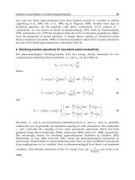
Figure 4 shows the first and second eigenvalues measured by the proposed method as a
function of the frame number in 2×2 MIMO system, where these eigenvalues are obtained

by using channel matrix and the transmit and receive weights determined by the proposed
algorithm. Figure 4 also shows eigenvalues determined by the SVD method. In Fig. 4,
although the first eigenvalue obtained by the proposed method occasionally takes slightly
smaller value than that of SVD, the proposed method finds almost the same eigenvectors as
the theoretical value obtained by SVD.
Figure 5 shows BER performance of N
t
x2 MIMO diversity system using the maximum ratio
combining (MRC) as a function of transmit signal to noise power ratio, where average gain
of channel is unity. Figure 6 also shows BER performance of 2xN
r
MIMO MRC diversity
system. In Figs. 5 and 6, the data stream is transmitted by the first eigenpath. Therefore, it
can be seen that both methods (LMS, SVD) achieve almost the same BER performance. This
result suggests that the eigenvector corresponding to the highest eigenvalue is correctly
detected as the first weight vector, i.e., the first eigenpath. It can be also qualitatively
explained that the highest eivenvalue is first found as the most dominant parameter
determining the error signal.
Figures 7 and 8 show BER performance of N
t
×2 and 2×N
r
E-MIMO, respectively. The number
of data streams is set to two, since the rank of channel matrix is two. Based on the BER
minimization criterion [1], the achievable BER is minimized by multiplying the transmit signal
by the inverse of the corresponding eigenvalue at the transmitter. In Figs. 7 and 8, we can see
that both methods (LMS and SVD) achieve almost the same BER performance.
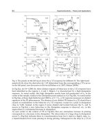
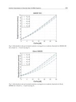
Figures 9 and 10 show the MIMO channel capacity in case of two data streams. In this paper,
for simplicity, MIMO channel capacity is defined as the sum of each eigenpath channel
capacity which is calculated based on Shannon channel capacity in AWGN channel [3];

C = log
2
(1+SNR) [bit/s/Hz] (17)
MIMO Systems, Theory and Applications

272
The transmit power allocation for each eigenpath is determined based on the water-filling
theorem [3]. In Figs.9 and 10, it can be seen that the E-SDM system with the proposed
method achieves the same channel capacity as that of the ideal one (SVD).



Fig. 4. Measured eigenvalues



Fig. 5. Bit error rate performance (1 data stream, N
t
×2)
Iterative Optimization Algorithms to Determine Transmit and Receive Weights for MIMO Systems

273





Fig. 6. Bit error rate performance (1 data stream, 2×N
r
)

Fig. 7. Bit error rate performance (2 data stream, N
t
×2)
MIMO Systems, Theory and Applications

274





Fig. 8. Bit error rate performance (2 data stream, 2×N
r
)





Fig. 9. Channel capacity performance (N
t
×2)
Iterative Optimization Algorithms to Determine Transmit and Receive Weights for MIMO Systems

275

Fig. 10. Channel capacity performance (2×N
r
)
3. Iterative optimization of the transmitter weights under constraint of the
maximum transmit power for an antenna element in MIMO systems
3.1 System model
Figure 11 shows MU-MIMO system considered in this paper, where K antenna elements
and single antenna element are equipped at the Base Station (BS) and Mobile Station (MS),
respectively. Single antenna is assumed for each Mobile Station (MS). The number of users
in SDMA is N. The receive signal at receive antenna Y=[y
1
, ⋅ ⋅ ⋅ ,y
N
]
T
is expressed as

HH H
rt r
=+YWHWXWn (18)
where superscript
T
and superscript
H
denote transpose and Hermitian transpose,
respectively. H is N×K complex channel metrics, W
t
is N×K complex transmit weight

matrices, W
r
=diag(w
1
, ⋅ ⋅ ⋅, w
N
) is receive weight metrics, X=[x
1
, ⋅ ⋅ ⋅,x
N
]
T
is transmit signal,
and μ=[n
1
, ⋅ ⋅ ⋅,n
N
]
T
is noise signal. The average power of transmit signal is unity (i.e., E[x
i
2
]
=1), where E[ ] denotes ensemble average operation) and there is no correlation between
each user signal (i.e., E[x
i1
x
i2
] =0), the condition to keep the total average transmit power to
be less than or equal to P

th
is given as

2
11
NK
i
j
th
ij
wP
==
≤
∑∑
(19)
where
w
ij
denotes the transmit weight of antenna #j for user #i. Then, the condition to
constrain the average transmit power per each antenna to be less than or equal to p
th
is
given as
MIMO Systems, Theory and Applications

276

2
1
N

i
j
th
i
wp
=
≤
∑
j
∀
(1
≤
j
≤
K) (20)

Base Station
Maximum permissible transmit
power per antenna:
th
p
#1
#K
H
User #1
User #N
Base Station
Maximum permissible transmit
power per antenna:
th

p
Maximum permissible transmit
power per antenna:
th
p
#1
#K
H
User #1
User #N

Fig. 11. MU-MIMO Systems

・・・
・・・・
H
H
t
W
r
W
ˆ
Base Station
User #1
1
n
1
w
1
ˆ

n
N
n
ˆ
1
x
N
x
1
ˆ
y
N
y
ˆ
1
y
#1
#K
Virtual Channel
& Receiver
Root Nyquist
Filter
Modulated
Signal
Root Nyquist
Filter
Modulated
Signal
Root Nyquist
Filter

Root Nyquist
Filter
weight
control
Root Nyquist
Filter
User #N
N
n
N
w
N
y
Root Nyquist
Filter
・・・
・・・・
H
H
t
W
r
W
ˆ
Base Station
User #1
1
n
1
w

1
ˆ
n
N
n
ˆ
1
x
N
x
1
ˆ
y
N
y
ˆ
1
y
#1
#K
Virtual Channel
& Receiver
Root Nyquist
Filter
Modulated
Signal
Root Nyquist
Filter
Modulated
Signal

Root Nyquist
Filter
Root Nyquist
Filter
weight
control
Root Nyquist
Filter
User #N
N
n
N
w
N
y
Root Nyquist
Filter

Fig. 12. System configurations

Pilot
Data
symbolsN
p
symbolsN
d
Pilot
Data
symbolsN
p

symbolsN
d

Fig. 13. Frame format
3.2 Transmitter and receiver model
Figure 12 shows the system configuration of the transmitter and receiver in MU-MIMO
system considered in this paper, where the number of transmit antennas and the number of
receive antennas are K and 1, respectively. A virtual channel and virtual receiver are
equipped with the transmitter to estimate mean square error at the receiver side, where
Iterative Optimization Algorithms to Determine Transmit and Receive Weights for MIMO Systems

277
ˆ
r
W
=diag(
1
ˆ
w,
⋅ ⋅ ⋅ ,
ˆ
w
N
) and
ˆ
n =[
1
ˆ
n , . . . ,
ˆ

n
N
]
T
denote the virtual receive weight and the
virtual noise, respectively. We assume that the average power of additive white Gaussian
noise (AWGN) is known to the transmitter, i.e., we assume
2
i
ˆ
nE
⎡
⎤
⎣
⎦
=E[n
i
2
]. Then, the receive
signal at the virtual receiver
ˆ
Y
is given as

ˆ
ˆˆ
ˆ
HH H
rt r
=+YWHWXWn

(21)
The transmit weights are optimized by minimizing the error signal between transmit and
receive signals at the virtual receiver under constraints given as Eqs.(19) and (20). Figure 13
shows a frame format assumed in this paper, where each frame consists of N
p
pilot symbols
and N
d
data symbols. Pilot symbols are known and used for optimizing the receive weights
on the receiver side.
3.3 Weight optimization
a. Problem Formulation
The transmit weights are optimized by minimizing the mean square error between transmit
and receive signals at the virtual receiver under constraint given as Eqs. (19) and (20). From
Eq.(21), the error signal between transmit signal X and receive signal at the virtual receiver
ˆ
Y
is given as

ˆ
ˆˆ
ˆ
HH H
rt r
e =−=− −XYXWHWXWn (22)
where e=[e
1
, . . . ,e
N
]. From Eqs.(19) and (20), the problem to minimize the mean square error

under two constraints can be formulated as the following constrained minimizing problem;
Minimize
2
()Ee
⎡
⎤
⎢
⎥
⎣
⎦
W

Subject to
2
11
() 0
NK
ij th
ij
gwP
==
=
−≤
∑∑
W
(23)

2
1
() 0

N
jijth
i
hwp
=
=
−≤
∑
W j
∀

where
⋅
denotes vector norm. W
is N×(N+K) complex matrix defined as W=[W
t
,
ˆ
r
W
].
b.
A EIPF based Approach for Weight Optimization
By introducing the extended interior penalty function (EIPF) method into the problem
shown in Eq.(23), this problem can be transformed into the following non-constrained
minimizing problem [11];
Minimize
{}
2
() () ()Ee r

⎡⎤
+Φ +Ψ
⎢⎥
⎣⎦
W
WW
Subject to
2
1
()
2()
if ( )
()
if ( )
g
g
g
g
ε
ε
ε
ε
−
⎧
−
≤
⎪
Φ=
⎨
−

>
⎪
⎩
W
W
W
W
W

MIMO Systems, Theory and Applications

278

1
() ()
K
j
j
ψ
=
Ψ=
∑
W
W

2
1
j
()
2()

j
if ( )
()
if ( )
j
j
h
j
h
h
h
ε
ε
ε
ψ
ε
−
⎧
−
≤
⎪
=
⎨
⎪
−
>
⎩
W
W
W

W
W

Here, ε(<0) and r(>0) denote the design parameters for non-constrained problem. In Eq.(24),
()Φ
W
and ()Ψ
W
increase rapidly as approaches to the boundary. When g(W) = ε and
h
j
(W)=ε, the continuity of ()
Φ
W
and ()
Ψ
W
is guaranteed as well as derivatives of these
two functions. Thus, Eq. (24) can be minimized by using the Steepest Descent method; W is
updated as

{}
2
(1) () () ()()mmEer
μ
⎛⎞
⎡⎤
+= −∇ +Φ +Ψ
⎜⎟
⎢⎥

⎣⎦
⎝⎠
WWwW WW
(28)
where μ is a step size to adjust the updating speed.
∇
w denotes a gradient with respect to
W, which is defined as

11 1 1
1
ˆ
ˆ
K
NNK N
www
ww w
⎡
⎤
∂∂∂
⎢
⎥
∂∂∂
⎢
⎥
⎢
⎥
∇=
⎢
⎥

∂∂ ∂
⎢
⎥
⎢
⎥
∂∂ ∂
⎣
⎦
W
0
0
"
#%# %
"
(29)
where j denotes an imaginary unit and

{}{}
Re() Im()
ij
i
j
i
j
j
w
ww
∂∂ ∂
=+
∂

∂∂
, (30)

{}{}
ˆˆ ˆ
Re() Im()
ii i
j
ww w
∂∂ ∂
=+
∂∂ ∂
, (31)
When
W is updated as in Eq. (28) at every symbols, Eq. (28) can be reduced to

{}
2
(1) () () ()()mm r
μ
⎡
⎤
+= −∇ +Φ +Ψ
⎢
⎥
⎣
⎦
W
WW eW WW. (32)
3.4 Performance evaluation

Performance of MU-MIMO system using the considered algorithm is evaluated by
computer simulation. Simulation parameters are shown in Table 2. As a channel model, we
consider a set of 8 plane waves transmitted in random direction within the angle range of 12
degrees at the BS. Each of the plane waves has constant amplitude and takes the random
phase distributed from 0 to 2π. All users are randomly distributed with a uniform
distribution in a range of the coverage area of a BS. Channel states and distribution of users
Iterative Optimization Algorithms to Determine Transmit and Receive Weights for MIMO Systems

279
change independently at every frame. Transmit weights are determined with recursive
calculation given in Eq.(32). Receive weights are determined by observing the pilot symbols.
The upper limit of the average transmit power for an antenna element normalized by the
upper limit of the total transmit power is denoted as

th
th
p
P
γ
= , (33)
where

1
1
K
γ
≤
≤ (34)
In Eq.(34), γ=1 corresponds to the case without constraint of per-antenna transmit power.
The minimum value of γ

is 1/K which corresponds to, the strictest case where per-antenna
transmit power is limited within the minimum value. The maximum permissible power per
user (P
th
/N) to noise power ratio is defined as

max
2
[]
SNR
th
i
P/N
E|n|
= (35)
where E[n
i
2
] denotes the average noise power corresponding to the user #i.

Channel Model Flat uncorrelated quasistatic Rayeigh fading
Modulation Method QPSK
Number of Pilot Symbols (N
p
) 34 [symbols/frame]
Number of Data Symbols (N
d
) 460 [symbols/frame]
Average propagation loss 0 [dB] (Except for Figs.20 and 21)
Antenna element spacing 5.25λ

Table 2. Simulation Parameters
Figures 14(a) and (b) show complementary cumulative distribution function (CCDF) of
average transmit power of transmit signal measured at every frames with respect to antenna
#1. The number of transmit antennas is set to 4 and 8, respectively. The number of users is 2.
The maximum permissible transmit power is set to P
th
=1.0, and average noise power is set
to E [n
i
2
]=0.1. From these figures, we can see that transmit power of the signal at antenna #1
can be kept below p
th
.
Figures 15 and 16 show the received SINR as a function of γ, where SNR
max
is set to 10 dB.
Note that SINR is the same as SNR when the number of users is 1. In these figures, we can
see that the degradation in SINR at γ=1/K is about 0.5dB and 0.6
～1.0dB for K=4 and 8 as
compared with the case of γ =1. It is shown that SINR is slightly degraded when γ ≤ 0.4 and
γ ≤ 0.3 for K=4 and K=8, respectively. This is because the probability that transmit power of
the signal at a certain antenna element exceeds γ becomes low as γ increases. The received
SINR is degraded as the number of users increases, because the diversity effect is reduced
attributable to the decrease of a degree of freedom on the number of antennas.
MIMO Systems, Theory and Applications

280
Figures 17 and 18 show BER performance as a function of SNR
max

, where the number of
users is set to 1∼3 for K=4 in Fig.17, and set to 3 for K=8 in Fig.18. In these figures, we can
see that, when the maximum per-antenna transmit power is limited to 1/K, BER
performances is degraded by about 0.7∼0.8 dB at BER=10
-2
as compared with case of γ=1.




(a) K=4, N=2



(b) K=8, N=2

Fig. 14. CCDF of average transmit power of the signal measured at every frames with
respect to antenna #1
Iterative Optimization Algorithms to Determine Transmit and Receive Weights for MIMO Systems

281








Fig. 15. SINR vs. γ (K=4, SNR

max
=10dB)








Fig. 16. SINR vs. γ (K=8, SNR
max
=10dB)
MIMO Systems, Theory and Applications

282






Fig. 17. Bit Error Rate Performance (K=4)






Fig. 18. Bit Error Rate Performance (K=8, N=3)

Iterative Optimization Algorithms to Determine Transmit and Receive Weights for MIMO Systems

283
4. Conclusion
We proposed optimization algorithms of transmit and receive weights for MIMO systems,
where the transmitter is equipped with a virtual MIMO channel and virtual receiver to
calculate the transmitter weight. First, we proposed an iterative optimization of transmit
and receive weights for E-SDM systems, where a least mean square algorithm is used to
determine the weight coefficients. The proposed method can be easily extended to the case
of E-SDM in MIMO system with arbitrary number of transmit and receive antennas. Second,
we proposed a weight optimization method of MIMO systems under constraints of the total
transmit power for all antenna elements and the maximum transmit power for an antenna
element. The performance of the proposed method is evaluated for QPSK signal in MU-
MIMO system with K antenna elements on the transmitter side and single antenna element
at the receive side. It is clarified that the degradation of received SINR attributable to
constraint of per antenna power is 0.5∼1.0 dB in case where the maximum transmit power
for an antenna element is limited to 1/K for the number of antenna of K=4 and 8. These
results mean that the proposed optimization algorithm enables to use a low cost power
amplifier at base stations in MIMO systems.
5. References
[1] T. Ohgane, T. Nishimura, & Y. Ogawa. Applications of Space Division Multiplexing and
Those Performance in a MIMO Channel, IEICE Transactions on Communications,
vol.E88-B, no.5, pp.1843-1851, May. 2005.
[2] G. Lebrun, J. Gao, & M. Faulkner. MIMO Transmission Over a Time-Varying Channel
Using SVD, IEEE Transactions on Wireless Communications, vol. 4, No.2, pp. 757 764,
March 2005.
[3] J. G. Proakis. Digital Communications, Fourth Edition, McGraw-Hill, 2001.
[4] S. Haykin. Adaptive Filter Theory, Fourth Edition, Prentice Hall, 2002.
[5] H. Yoshinaga, M.Taromaru, & Y.Akaiwa. Performance of Adaptive Array Antenna with
Widely Spaced Antenna Elements, Proceedings of the IEEE Vehicular Technology

Conference Fall'99, pp.72-76, Sept. 1999.
[6] T. Nishimura, Y. Takatori, T. Ohgane, Y. Ogawa, & K. Cho, Transmit Nullforming for a
MIMO/SDMA Downlink with Receive Antenna Selection, Proceedings of the IEEE
VTC Vehicular Technology Conference Fall’02, pp.190-194, Sept. 2002.
[7] Y. Kishiyama, T. Nishimura, T. Ohgane, Y. Ogawa, & Y. Doi. Weight Estimation for
Downlink Null Steering in a TDD/SDMA System, Proceedings of the IEEE VTC
Vehicular Technology Conference Spring'00, pp.346-350, May 2000.
[8] Y. Doi, Tadayuki Ito, J. Kitakado, T. Miyata, S. Nakao, T. Ohgane, & Y. Ogawa. The
SDMA/TDD Base Station for PHS Mobile Communication, Proceedings of the IEEE
Vehicular Technology Conference Spring'02, pp.1074-1078, May 2002.
[9] T. Nishimura, T. Ohgane, Y. Ogawa, Y. Doi, & J. Kitakado. Downlink Beamforming
Performance for an SDMA Terminal with Joint Detection, Proceedings of the IEEE
Vehicular Technology Conference Fall'01, pp.1538-1542, Oct. 2001.
[10] B. S. Krongold. Optimal MIMO-OFDM Loading with Power-Constrained Antennas,
Proceedings of the IEEE PIMRC'06, Sept. 2006.
MIMO Systems, Theory and Applications

284
[11] S. S. Rao. Engineering Optimization, Theory and Practice, 3rd Edition, Wiley-Interscience,
1996.
0
Beamforming Based on Finite-Rate Feedback
Pengcheng Zhu
1
, Lan Tang
2
, Yan Wang
3
, Xiaohu You
4

1,3,4
National Mobile Communications Research Laboratory
Southeast University, Nanjing, 210096
4
School of Electrical Science and Engineering
Nanjing University, Nanjing, 210093
P. R. China
1. Introduction
Multiple-input multi-output (MIMO), emerged as one of the most significant breakthroughs
in wireless communications theory over the last two decades, is considered as a key to meeting
the increasing demands for high data rates and mass wireless access services over a limited
spectrum bandwidth. Transmit beamforming with receive combining is a low-complexity
technique to exploit the benefits of MIMO wireless systems. It has received much interest
over the last few years, because it provides substantial performance improvement without
sophisticated signal processing. In order to enable the beamforming operation, either full or
partial channel state information (CSI) has to be furnished to the transmitter. With full CSI,
the optimal transmit beamforming scheme is maximum ratio transmission (MRT) [Dighe et
al. (2003a)], where the principal right singular vector of the channel matrix is used as the
beamforming vector. In Rayleigh fading, exact expressions for the symbol error rate (SER)
of MRT were derived in [Dighe et al. (2003a;b)], and the asymptotic error performance was
studied in [Zhou & Dai (2006)].
However, in certain application scenarios, e.g. frequency division duplex (FDD) systems,
CSI is not usually available at the transmitter. To cope with the lack of CSI, a beamforming
scheme based on finite-rate feedback has been proposed in the literature, where the CSI is
quantized at the receiver and fed back to the transmitter. This scheme has been adopted
in current 3GPP specifications. Under the assumption of independent block-fading and
the assumption of delay- and error-free feedback, the design and performance analysis of
quantized beamforming systems have been well investigated. Different beamformer design
methods were developed in [Mukkavilli et al. (2003); Love & Heath (2003); Xia & Giannakis
(2006)]. In multiple-input single-output (MISO) cases, lower bounds to the outage probability

and symbol error rate (SER) were derived in [Mukkavilli et al. (2003)] and [Zhou et al. (2005)],
respectively. In MIMO cases, the average receive signal-to-noise ratio (SNR) and outage
probability were studied in [Mondal & Heath (2006)]. Analytical results showed that full
diversity order can be achieved by a well-designed beamformer [Love & Heath (2005)].
This chapter highlights recent advances in beamforming based on finite-rate feedback from a
communication-theoretic perspective. We first study the SER performance when the feedback
link is delay- and error-free. Then non-ideal factors in the feedback link are investigated, and
countermeasures are proposed to compensate the performance degradation due to non-ideal
feedback.
12
Coding &
Modulation
s


Beamformer
w
1
w
N
t


z
1
Combiner
r
Detection &
Decoding
H

Ideal channel
estimation
Codeword
selection
Feedback channel
z
N
r
H
wz
Index
Beamforming
vector update
Fig. 1. A beamforming system based on finite-rate feedback.
The notations used in this chapter are conformed to the following convention. Bold upper
and lower case letters are used to denote matrices and column vectors, respectively.
(·)
T
, and
(·)
∗
refer to transpose and conjugate transpose, respectively. ·and ·
F
stand for vector
2-norm and matrix Frobenius norm, respectively. I
N
refers to the N × N identity matrix.
CN (μ, σ
2
) stands for the circularly symmetric complex Gaussian distribution with mean μ

and covariance σ
2
.Prand denote the probability and expectation operators, respectively.
2. An upper bound on the SER
In this section, we evaluate the SER of a beamforming system based on finite-rate feedback.
Assuming a delay- and error-free feedback link, we derive an upper bound on the average
SER, and prove that the bound is asymptotically tight in high SNR regions.
2.1 System model
Consider an MIMO system with N
t
transmit and N
r
receive antennas. The wireless channel is
assumed to be frequency-flat, and is modeled as an N
r
× N
t
random matrix H. The (m, n)-th
entry of the channel matrix, h
m,n
, denotes the fading coefficient between the n-th transmit
antenna and the m-th receive antenna. We assume an independent and identically distributed
(i.i.d.) Rayleigh fading. Then the fading coefficient h
m,n
’s are independent of each other and
distributed as
CN (0, 1).
The system adopts transmit beamforming with receive combining, as shown in Figure 1.
At the transmitter, the information-bearing symbol s
∈ is weighted by a beamforming

vector, and transmitted simultaneously from all antennas. Then the N
t
×1 transmitted signal
vector is given by x
= w s, where w =[w
1
, ···, w
N
t
]
T
denotes the beamforming vector. The
beamforming vector is a unit-norm vector, satisfying
w = 1. At the receiver, the N
r
× 1
received signal vector can be expressed as
y
= Hw s + η, (1)
where η refers to the noise vector with independent
CN (0, N
0
) entries. Assuming that the
receiver knows the channel H and the beamforming vector w, it performs receive combining
286
MIMO Systems, Theory and Applications
to the received signal, using the maximum ratio combining (MRC) vector [Love & Heath
(2003)]
z
=

Hw
Hw
.
The signal r
∈ after receive combining can be written as
r
= z
∗
y = z
∗
Hw s + z
∗
η, (2)
and the corresponding instantaneous receive SNR is given by
γ
= γ
S
Hw
2
, (3)
where
γ
S
 (|s|
2
)/N
0
(4)
is the average symbol SNR.
In a beamforming system based on finite-rate feedback, the beamforming vector w is restricted

to lie in a finite set (codebook) that is known to both the transmitter and receiver. The
codebook, denoted as
C, is designed in advance and consists of N
c
= 2
B
unit-norm codewords
C = {c
1
, ···, c
N
c
}. The receiver selects the favorable codeword from the codebook according
to
c
opt
= arg max
c∈C
Hc
2
. (5)
If the codeword c
k
is selected (c
opt
= c
k
), its index k is sent to the transmitter via a feedback
link, requiring B bits each time. In this section, we focus on the case of delay- and error-free
feedback. The transmitter obtains the index of the optimal codeword, and uses the codeword

as beamforming vector. Then we have
w
= c
opt
(delay- and error-free feedback). (6)
As in [Love & Heath (2005)], we assume the beamforming codewords
{c
1
, ···, c
N
c
} span
N
t
.
This property guarantees the soundness of several steps in the following derivation. We note
that it is a mild condition. To our knowledge, all well-designed codebooks, e.g. those in [Love
& Heath (2003); Xia & Giannakis (2006)] and 3GPP specifications, satisfy this condition.
2.2 SER analysis
For notation brevity, phase-shift keying (PSK) signals are assumed in the derivations.
Conditioned on the instantaneous SNR γ, the SER of M-ary PSK can be expressed as [Simon
& Alouini (2005), Eq.(8.23)]
P
E
=
1
π

(M−1)π
M

0
exp

−
g
PSK
γ
sin
2
θ

dθ, (7)
where g
PSK
= sin
2
(π/M) is a constellation-dependent constant. Applying (6) and (5) to (3),
the instantaneous SNR of the beamforming system is given by
γ = γ
S
Hw
2
= γ
S
Hc
opt

2
= γ
S

max
c∈C
Hc
2
(8)
Then substituting (8) into (7) and taking expectation, the average SER of the beamforming
system can be written as
P
E
 P
E
=
1
π

(M−1)π
M
0
exp

−
g
PSK
γ
S
sin
2
θ
max
c∈C

Hc
2

dθ, (9)
287
Beamforming Based on Finite-Rate Feedback
where the expectation is respect to the channel matrix H.
To find an upper bound on the average SER, we first study the expectation term in the
right-hand-side of (9), as shown in the following lemma.
Lemma 1. Let H be an N
r
× N
t
random matrix with i.i.d. CN (0, 1) entries, and define
˜
H
 H/H
F
.
Then for a given beamforming codebook
C, and a given t ≥ 0, we have
exp

−t ·max
c∈C

Hc

2


≤

1
+ t ·g
CB

−N
t
N
r
, (10)
where
g
CB

 

max
c∈C

˜
Hc

2

−N
t
N
r


−
1
N
t
N
r
(11)
is a codebook-dependent parameter.
Proof: Since the channel matrix H has i.i.d.
CN (0, 1) entries, H
2
F
is chi-square distributed
and independent of
˜
H . The moment generating function of
H
2
F
is given by
exp

−sH
2
F

=(1 + s)
−N
t
N

r
. (12)
Therefore we have
exp

−t ·max
c∈C
Hc
2

=


exp

−t ·H
2
F
·max
c∈C

˜
Hc

2




˜

H


=


1
+ t ·max
c∈C

˜
Hc

2

−N
t
N
r

. (13)
Notice that when x, t
> 0,
f
(x)=

1
+ t · x
−
1

N
t
N
r

−N
t
N
r
is a concave function with respect to x. We can apply Jensen’s inequality to the right-hand-side
of (13), and obtain


1
+ t ·max
c∈C

˜
Hc

2

−N
t
N
r

=

1

+ t ·


max
c∈C

˜
Hc

2

−N
t
N
r
  
treated as a r. v.

−
1
N
t
N
r

−N
t
N
r


≤

1
+ t ·
 

max
c∈C

˜
Hc

2

−N
t
N
r

−
1
N
t
N
r

−N
t
N
r

. (14)
Substituting this into (13), we reach the desired result (10).

In Lemma 1, the definition of g
CB
is not given in a closed-form. Its value has to be evaluated
numerically. In the following lemma, we will further study the parameter, and derive a
closed-form approximation for it.
Lemma 2. The parameter g
CB
satisfies 0 ≤ g
CB
≤ 1.Moreover, for a well-designed codebook, it can
be approximated by
g
−N
t
N
r
CB
 N
c
C
1
(N
t
N
r
−1)! (N
t

−1)
N
t
−2
∑
n= 0

N
t
−2
n

(−1)
n
(C
−(N
t
N
r
−1−n)
2
−1)
N
t
N
r
−1 − n
, (15)
288
MIMO Systems, Theory and Applications

where
C
1
 N
t
N
r
min
(N
t
,N
r
)
∏
n= 1
[min(N
t
, N
r
) − n]!
(N
t
+ N
r
−n)!
(16)
and
C
2
 1 −


1/N
c

1
N
t
−1
. (17)
Proof: We first prove 0
≤ g
CB
≤ 1. It is clear from the definition that g
CB
≥ 0. To see g
CB
≤ 1,
consider the following equality
lim
t→∞
t
N
t
N
r


1
+ t ·max
c∈C


˜
Hc

2

−N
t
N
r

=

lim
t→∞
t
N
t
N
r

1
+ t ·max
c∈C

˜
Hc

2


−N
t
N
r

=


max
c∈C

˜
Hc

2

−N
t
N
r

. (18)
By the definition (11), (18) implies that
g
−N
t
N
r
CB
= lim

t→∞
t
N
t
N
r


1
+ t ·max
c∈C

˜
Hc

2

−N
t
N
r

(19)
Notice that

˜
H

F
= 1 and c = 1, ∀c ∈C. Therefore

max
c∈C

˜
Hc

2
≤ 1
and


1
+ t ·max
c∈C

˜
Hc

2

−N
t
N
r

≥ (1 + t )
−N
t
N
r

.
So we have
g
−N
t
N
r
CB
= lim
t→∞
t
N
t
N
r


1
+ t ·max
c∈C

˜
Hc

2

−N
t
N
r


≥ lim
t→∞
t
N
t
N
r
(1 + t)
−N
t
N
r
= 1 , (20)
which implies β
C
≤ 1.
To obtain (15), recall Equation (13) in the proof of Lemma 1. Substituting it into (19) yields
g
−N
t
N
r
CB
= lim
t→∞
t
N
t
N

r
exp

−t ·max
c∈C
Hc
2

. (21)
Let the eigen-decomposition of the channel be denoted as
H
∗
H =

u
1
, ···, u
N
t

⎡
⎢
⎣
λ
1
.
.
.
λ
N

t
⎤
⎥
⎦
⎡
⎢
⎣
u
∗
1
.
.
.
u
∗
N
t
⎤
⎥
⎦
(22)
where λ
1
≥···≥λ
N
t
≥ 0 and u
1
, ···, u
N

t
denote the eigenvalues and the eigenvectors,
respectively. We have the following inequality
Hc
2
= c
∗
H
∗
Hc =
N
t
∑
n= 1
λ
n
|u
∗
n
c|
2
≥ λ
1
|u
∗
1
c|
2
. (23)
289

Beamforming Based on Finite-Rate Feedback
Substituting (23) into (21), one obtains
g
−N
t
N
r
CB
≤ lim
t→∞
t
N
t
N
r
exp

−tλ
1
·max
c∈C
|u
∗
1
c|
2

. (24)
In an i.i.d. Rayleigh fading scenario, H
∗

H is Wishart distributed. The eigenvalue and
eigenvector of a Wishart matrix are independent of each other. So (24) can be expressed as
g
−N
t
N
r
CB
≤ lim
t→∞
t
N
t
N
r



∞
0
e
−txz
p
λ
1
(x) dx

d

Pr


max
c∈C
|u
∗
1
c|
2
< z

=


lim
t→∞
t
N
t
N
r

∞
0
e
−txz
p
λ
1
(x) dx


d

Pr

max
c∈C
|u
∗
1
c|
2
< z

(25)
Since H
∗
H is Wishart distributed, the probability density function (PDF) of its largest
eigenvalue λ
1
has the asymptotic property [Zhou & Dai (2006)]
p
λ
1
(x)=C
1
x
N
t
N
r

−1
+ o(x
N
t
N
r
−1
), x → 0
+
, (26)
where C
1
is defined in (16), and o(x
N
t
N
r
−1
) stands for a function a(x) satisfying
lim
x→0
+
a(x)/x
N
t
N
r
−1
= 0. Then we have
lim

t→∞
t
N
t
N
r

∞
0
e
−txz
p
λ
1
(x) dx = lim
t→∞
t
N
t
N
r

∞
0
e
−yz
p
λ
1
(y/t) d(y/t )

=

∞
0
e
−yz

lim
t→∞
t
N
t
N
r
−1
p
λ
1
(y/t)

dy
=

∞
0
e
−yz
C
1
y

N
t
N
r
−1
dy
= C
1
(N
t
N
r
−1)! z
−N
t
N
r
(27)
Substituting (27) into (25) yields
g
−N
t
N
r
CB
≤ C
1
(N
t
N

r
−1)!

z
−N
t
N
r
d

Pr

max
c∈C
|u
∗
1
c|
2
< z

. (28)
For a well-designed codebook, the Voronoi cells of the codewords can be approximated by
’spherical caps’, which leads to a very tight bound [Zhou et al. (2005)]
Pr

max
c∈C
|u
∗

1
c|
2
< z

≥ 1 − N
c
(1 − z)
N
t
−1
, C
2
≤ z ≤ 1, (29)
where C
2
is defined in (17). The inequalities (28) and (29) are both tight. We now treat
then as approximations, and substitute (29) into (28). After performing the integration, the
right-hand-side of (15) is obtained.

We then apply the results in Lemma 1 and 2 to the SER analysis. Setting t = g
PSK
γ
S
/ sin
2
θ
and after some manipulations, (10) becomes
exp


−
g
PSK
γ
S
sin
2
θ
max
c∈C
Hc
2

≤

sin
2
θ
g
PSK
g
CB
γ
S
+ sin
2
θ

N
t

N
r
. (30)
Substituting this into (9), we obtain an upper bound on the average SER of M-ary PSK signal
P
E
≤ P
ub
E
=
1
π

(M−1)π
M
0

sin
2
θ
g
PSK
g
CB
γ
S
+ sin
2
θ


N
t
N
r
dθ, (31)
290
MIMO Systems, Theory and Applications
which is the main result of this section.
At last, we give two remarks on the SER bound.
Remark 1 (Asymptotic behavior). The upper bound has the merit of being asymptotically
tight. In fact, at high SNR, we have
G
= lim
γ
S
→∞
γ
N
t
N
r
S
P
E
(9)
=
1
π
lim
γ

S
→∞
γ
N
t
N
r
S

(M−1)π
M
0
exp

−
g
PSK
γ
S
sin
2
θ
max
c∈C
Hc
2

dθ
=
1

π

(M−1)π
M
0

sin
2
θ
g
PSK

N
t
N
r

lim
γ
S
→∞

g
PSK
γ
S
sin
2
θ


N
t
N
r
exp

−
g
PSK
γ
S
sin
2
θ
max
c∈C
Hc
2


dθ
(21)
=
1
π

(M−1)π
M
0


g
PSK
γ
S
sin
2
θ

N
t
N
r
(g
CB
)
−N
t
N
r
dθ
=
1
π

(M−1)π
M
0
(sin θ)
2N
t

N
r
(g
PSK
g
CB
)
N
t
N
r
dθ . (32)
This equation shows that as γ
S
→ ∞, P
E
decreases as Gγ
−N
t
N
r
S
+ o(γ
−N
t
N
r
S
). G
−1

N
t
N
r
is usually
referred to as the coding gain. On the other hand, it is easily verified that
lim
γ
S
→∞
γ
N
t
N
r
S
P
ub
E
= G .
Therefore, (31) is asymptotically tight at high SNR. Moreover, when γ
S
= 0, both sides of (31)
are equal to
(M − 1)/M. So the bound holds with equality. This guarantees the tightness of
the bound at low SNR.
Remark 2 (Extension to other constellations). For brevity, we have assumed a phase-shift
keying (PSK) signal in the derivation of the SER bound. However, the same procedure can
be applied to other 2-D constellations. For example, the SER of square quadrature amplitude
modulation (QAM), conditioned on the instantaneous SNR γ, can be expressed as [Simon &

Alouini (2005)]
P
E,QAM
=
4(
√
M −1)
πM

π/4
0
exp

−
g
QAM
γ
sin
2
θ

dθ
+
4(
√
M −1)
π
√
M


π/2
π/4
exp

−
g
QAM
γ
sin
2
θ

dθ,
where M is the constellation size, and g
QAM
= 1.5/(M −1). This equation has a similar form
to (7). Using the procedure of deriving (31), we can obtain an upper bound on the average
SER of QAM
P
E,QAM
= P
E,QAM
≤
4(
√
M −1)
πM

π/4
0


sin
2
θ
g
QAM
g
CB
γ
S
+ sin
2
θ

N
t
N
r
dθ
+
4(
√
M −1)
π
√
M

π/2
π/4


sin
2
θ
g
QAM
g
CB
γ
S
+ sin
2
θ

N
t
N
r
dθ . (33)
291
Beamforming Based on Finite-Rate Feedback
2.3 Extension to correlated rayleigh fading
In a correlated Rayleigh fading channel, the system model is the same as in Section 2.1, except
that the channel matrix is modeled as
vec
(H)=Φ
Φ
Φh
w
, (34)
where h

w
refers to an N
t
N
r
× 1 random vector with independent CN (0, 1) entries; Φ
Φ
Φ is an
N
t
N
r
× N
t
N
r
positive definite matrix; and vec(H) denotes the N
t
N
r
× 1 vector of stacked
columns of H. Φ
Φ
Φ
2
(= Φ
Φ
ΦΦ
Φ
Φ

∗
) is usually called the channel correlation matrix.
The idea used in Section 2.2 can be extended to correlated Rayleigh fading scenarios. For
M-ary PSK signals, we can prove that the average SER is upper bounded by
P
E
≤
1
π

(M−1)π
M
0

sin
2
θ
g
PSK
g
CB
g
Cor
γ
S
+ sin
2
θ

N

t
N
r
dθ, (35)
where
g
Cor


det
(Φ
Φ
Φ
2
)

1
N
t
N
r
is a parameter depends on the channel correlation matrix. The proof of this bound is out
of the scope of this book. Interesting readers are referred to [Zhu et al. (2010)] for detailed
derivations.
The bound (35) is asymptotically tight at high and low SNRs [Zhu et al. (2010)]. However, at
medium SNR, the tightness of the bound is not guaranteed because it does not fully reflect
the effect of channel correlation. Based on extensive simulations, we propose the following
conjectured SER formula
P
E

conjectured
≤
1
π

(M−1)π
M
0
N
t
N
r
∏
i=1
sin
2
θ
g
PSK
g
CB
γ
S
λ
Φ
2
, i
+ sin
2
θ

dθ, (36)
where λ
Φ
2
, i
denotes the i-th eigenvalue of Φ
2
. We have not been able to prove the conjecture
as yet. Some discussion in support of it is presented in [Zhu et al. (2010)].
2.4 Numerical results
Simulations are carried out for 2Tx-2Rx and 4Tx-2Rx antenna configurations. QPSK and
16-QAM constellations are used in the simulations. The 2Tx-2Rx system uses the 2-bit
Grassmannian codebook ([Love & Heath (2003)]-TABLE II), and the 4Tx-2Rx system adopts
the 4-bit codebook in 3GPP specification ([3GPP TS 36.211 (2009)]-Table 6.3.4.2.3-2).
Figure 2 and 3 show the average SER in uncorrelated Rayleigh fading. The SER bounds (31)
(33) are tight in these figures.
We also consider a correlated Rayleigh fading channel. The channel correlation matrix Φ
2
is
generated according to the 802.11n model D [Erceg et al. (2004)]. We assume uniform linear
arrays with 0.5-wavelength adjacent antenna spacing, as in [Erceg et al. (2004), Section 7].
Figure 4 and 5 plot the average SER in this fading environment. In both figures, the gap
between the simulation result and the bound (35) is no more than 2 dB. The conjectured SER
formula (36) is even tighter than the bound.
292
MIMO Systems, Theory and Applications
0 3 6 9 12 15 18 21 24
10
−6
10

−5
10
−4
10
−3
10
−2
10
−1
10
0
Symbol SNR γ
S
(dB)
SER
2 Tx, 2 Rx, uncorrelated Rayleigh fading
Upper bound (31)
Upper bound (33)
SER of QPSK
SER of 16−QAM
Fig. 2. SER of the 2Tx-2Rx beamforming system in Rayleigh fading environment.
0 2 4 6 8 10 12 14 16 18 20
10
−6
10
−5
10
−4
10
−3

10
−2
10
−1
10
0
Symbol SNR γ
S
(dB)
SER
4 Tx, 2 Rx, uncorrelated Rayleigh fading
Upper bound (31)
Upper bound (33)
SER of QPSK
SER of 16−QAM
Fig. 3. SER of the 4Tx-2Rx beamforming system in Rayleigh fading environment.
293
Beamforming Based on Finite-Rate Feedback