GIÁO TRÌNH KHAI THÁC PHẦN mềm TRONG GIA CÔNG KHUÔN mẫu chapter VI flow rule
Bạn đang xem bản rút gọn của tài liệu. Xem và tải ngay bản đầy đủ của tài liệu tại đây (273.71 KB, 11 trang )
1
Chapter VI: Flow Rule
1
Content
• Terminology
• Elastic Stress-Strain Relationship
• Uniaxial Observations
• Levy-Mises Flow Rule
• Derivation of Equivalent Plastic Strain Rate
• Principle of Normality
• Work-Hardening Case
• Hoogenboom’s Experiment
Chapter VI: Flow Rule
2
Terminology
• Solid Mechanics: Stress-Strain Relationship (especially in
elasticity)
• Continuum Mechanics: Constitutive Equations, Material Law
• Plasticity: Flow Rule
The material dependent relationship between the stress and
the strain is described in literature by various terms:
2
Chapter VI: Flow Rule
3
Elastic Stress-Strain Relationships
For small strain elastic behaviour, the stress-strain relation is given by:
( )
( )
( )
0 0 0
0 0 0
0 0 0
0
0
0
1
1
1
1 1
2 2
1 1
2 2
1 1
2 2
xx xx yy zz
yy yy xx zz
zz zz xx yy
xy xy xy
yz yz yz
zx zx zx
e
E
e
E
e
E
e
G
e
G
e
G
σ ν σ σ
σ ν σ σ
σ ν σ σ
γ τ
γ τ
γ τ
= − +
= − +
= − +
= =
= =
= =
⇒
0
1
2
ij ij
e
G
σ
′ ′
=
( )
0
where,
is the engineering strain tensor
the deviatoric engineering strain tenso
r
the nominal stress tensor
the Young's modulus
the Poisson's ratio
the shear modulus and
2 1
ij
ij
ij
e
e
E
E
G G
σ
ν
ν
′
=
+
Chapter VI: Flow Rule
4
Uniaxial Observations
Consider the given
simple tension test:
1
1
2 3
0
0
3
h
σ
σ
σ
σ σ
≠
⇒ = ⇒
= =
λ
λλ
λ
F
F
d
λ
λλ
λ
1 1 2 3 1
1 2 3
2 1
,
3 3
2 2
σ σ σ σ σ
σ σ σ
′ ′ ′
= = = −
′ ′ ′
= − = −
Stress State:
Strain Increment State:
1 2 3
2 2
d d d
ε ε ε
= − = −
Hence:
1 2 3
1 2 3
d d d
d
ε ε ε
λ
σ σ σ
= = =
′ ′ ′
3
Chapter VI: Flow Rule
5
Levy-Mises Flow Rule (1)
These observations lead to the general Levy-Mises flow rule:
ij ij
d d
ε λ σ
′
= ⋅
where:
is the plastic true strain increment
the deviatoric true stress
a non-negative real number
ij
ij
d
d
ε
σ
λ
′
Remark: The Levy-Mises flow rule assumes rigid-plastic
deformation, i.e. ignores elastic deformations. Hence the first
invariant of the strain increment tensor is zero.
Chapter VI: Flow Rule
6
Levy-Mises Flow Rule (2)
ij ij
ε λ σ
′
= ⋅
&
&
By dividing both sides of the Levy-Mises equation by dt we obtain
an alternative form in terms of strain rates:
To determine the non-negative proportionality factor in the above
equation consider following development:
3 3
ij
1 1
3 3
1 1
3
with we obtain:
2
1 3
2
ij
ij ij
i j
ij ij
i j
ε
σ σ σ σ
λ
σ ε ε
λ
= =
= =
′ ′ ′
= =
=
∑∑
∑∑
&
&
& &
&
3 3
1 1
3
2
ij ij
i j
ε ε
λ
σ
= =
=
∑∑
& &
&
or:
4
Chapter VI: Flow Rule
7
Levy-Mises Flow Rule (3)
Notice that
3 3
2
1 1
1
2nd invariant of
2
ij
ij ij ij
i j
I
ε
ε ε ε
= =
≡ ≡
∑∑
&
& & &
Hence:
2
3
ij
I
ε
λ
σ
⋅
=
&
&
Furthermore, note that the material must be always in the plastic
state for above equation to hold, so that:
f
σ σ
→
and hence:
2
3
ij
f
I
ε
λ
σ
⋅
=
&
&
where
σ
f
is the so-called
flow stress.
Chapter VI: Flow Rule
8
Levy-Mises Flow Rule (4)
So, the Levy-Mises flow rule can be rewritten as:
2
3
ij
ij ij
f
I
ε
ε σ
σ
⋅
′
=
&
&
This equation can be further simplified by recalling the equivalent
plastic strain rate using the identity:
3 33 3
ij i ij i
j
j
ji i
j
p
σ
ε σ ε
εσ
= ⋅ ⋅=
′
= ⋅
∑∑ ∑∑
&
&
&
5
Chapter VI: Flow Rule
9
Derivation of the Equivalent Strain Rate (1)
Replacing in
3 3
ij ij
i j
σ ε σ ε
′
⋅ = ⋅
∑∑
&
&
2
3
ij
ij ij
f
I
ε
ε σ
σ
⋅
′
=
&
&
the strain rate tensor by:
we obtain:
3 3
2
3
ij
ij ij
i j
f
I
ε
σ ε σ σ
σ
⋅
′ ′
⋅ = ⋅
∑∑
&
&
Chapter VI: Flow Rule
10
Derivation of the Equivalent Strain Rate (2)
2
3 3
2
2
3
ij
ij ij
i j
f
J
I
ε
σ ε σ σ
σ
⋅
⋅
′ ′
⋅ = ⋅
∑∑
&
&
1442443
Or:
But recall that:
3 3
2
3
= = 3
2
f ij ij
i j
J
σ σ σ σ
′ ′
= ⋅ ⋅
∑∑
2
2
3
2
3
ij
f f
f
I
ε
σ ε σ
σ
⋅
⋅ =
&
&
6
Chapter VI: Flow Rule
11
Derivation of the Equivalent Strain Rate (3)
3 3
2
1 1
4 2
3 3
ij
ij ij
i j
I
ε
ε ε ε
= =
= ⋅ =
∑∑
&
&
& &
Hence:
So, the Levy-Mises flow rule can be rewritten finally as:
3
2
ij ij
f
ε
ε σ
σ
′
=
&
&
3
2
ij ij
f
d
d
ε
ε σ
σ
′
=
or, equivalently, as
Chapter VI: Flow Rule
12
Comparison of Hooke’s Law and Levy-
Mises Flow Rule
The Levy-Mises equation can be written also in terms of the total
stresses:
( )
1 1 2 3
1
etc.
2
f
d
d
ε
ε σ σ σ
σ
= − +
Comparing this form with the Hooke’s law:
( )
1 2 3
0 0 0
1
1
e
E
σ ν σ σ
= − +
Note:
1. The Poisson’s ratio is replaced by the factor 0.5 in the Levy-Mises law
2. The constant Young’s modulus is now a variable depending on the flow
stress and the equivalent plastic strain increment in the plastic case
3. Levy-Mises equations are relating stresses to strain increments or rates
7
Chapter VI: Flow Rule
13
Normality Rule (1)
In fact the Levy-Mises flow rule is one typical application of the
plastic potential theory, which establishes the flow rule by:
ij
ij
f
d d
ε λ
σ
∂
= ⋅
∂
where f is the so-called plastic potential. In case of associative
plasticity this potential is taken identical to the yield function.
Above equation indicates also that the strain increment “vector”
is normal to the yield surface in the stress space.
Chapter VI: Flow Rule
14
Normality Rule (2)
For the two-dimensional plane stress case the normality rule
can be illustrated by:
One important fact about flow surfaces is that they must be
convex always for stable material flow.
8
Chapter VI: Flow Rule
15
Work-Hardening Case
3
2
ij ij
f
d
d
ε
ε σ
σ
′
=
For non-hardening (perfect plastic) case we found:
For an hardening material according to the flow curve
( )
f
σ ε
we can define the local slope H as:
f f
d d
H d
d H
σ σ
ε
ε
= ⇒ =
Inserting the latter into the first equation above gives:
3
2
f
ij ij
f
d
d
H
σ
ε σ
σ
′
=
Chapter VI: Flow Rule
16
Work-Hardening Case: Ludwik Eqn.
n
f
C
σ ε
=
For a flow curve of Ludwik’s type:
(C and n are material constants)
we can find the slope as:
1
n
n
f f
d
H C n
d C
σ σ
ε
−
= = ⋅ ⋅
9
Chapter VI: Flow Rule
17
Remark on Levy-Mises Flow Rule
3
2
f
ij ij
f
d
d
H
σ
ε σ
σ
′
=
From the flow rule
it is apparent that:
has the same "direction" as and NOT !
ij ij ij
d
ε σ σ
′
In case of Hooke’s law:
has the same "direction" as !
ij ij
d
ε σ
′ ′
Chapter VI: Flow Rule
18
Hoogenboom’s Experiment (1)
Stan Hoogenboom (Ankara, 2002)
Experimental procedure:
1. Load the wire
with weights until
it elongates
plastically.
2. Keeping this
axial load, start
to apply a torque
to the wire by
rotating it.
10
Chapter VI: Flow Rule
19
Hoogenboom’s Experiment (2)
z
θ
τ
⇒
where m is the mass of
the weights, g the
gravitational accelaration
and A the current cross-
sectional arae of the wire.
z
m g
A
σ
⋅
=
due to the torque T
Chapter VI: Flow Rule
20
Hoogenboom’s Experiment (3)
The strain increment due to axial load is simply:
3 3 1
2 2 3
f f f
zz zz zz zz zz
f f f
d
d d d
d
H H H
λ
σ σ σ
ε σ σ σ σ
σ σ σ
′
= ⋅ = ⋅ − = ⋅
14243
Now, after the axial load is kept constant, the torque T is applied:
( )
after torque
1
2
f xx
σ σ
=
yy
σ
−
( )
2
yy
σ
+
( )
2
zz zz xx
σ σ σ
− + −
( )
2
2
6
xy
τ
+
2 2
yz zx
τ τ
+ +
(
)
Therefore:
(
)
(
)
(
)
after torque after torque before torque
0
f f f
d
σ σ σ
≈ − >
Hence:
0
f
zz zz
f
d
d
H
σ
ε σ
σ
= ⋅ >
during torque application
11
Chapter VI: Flow Rule
21
Examples (1)
Example 5.1:
The plane strain state of deformation is defined as that state for
which one of the three principal strain rates is zero for the whole
deformation. A typical plane strain state is given in case of the
flat rolling process. Here the strain in the width direction (parallel
to the roll axis) is approximately zero.
Describe the characteristic state of stress corresponding to a
plane strain state.
Chapter VI: Flow Rule
22
Examples (2)
Example 5.2:
Consider the uniform rod with current diameter D= 25 mm and
current length of λ = 120 mm, which is plastically deformed with
a velocity of v
tool
=3 mm/s at each end. If the material has a flow
stress of 250 MPa at the current strain, strain rate and
temperature, determine all the external forces acting on the
specimen.