Biosignal and Biomedical Image Processing MATLAB-Based Applications phần 10 pot

344 Chapter 12
both upper and lower boundaries, an operation termed slicing since it isolates a
specific range of pixels. Slicing can be generalized to include a number of dif-
ferent upper and lower boundaries, each encoded into a different number. An
example of multiple slicing was presented in Chapter 10 using the MATLAB
gray2slice
routine. Finally, when RGB color or pseudocolor images are in-
volved, thresholding can be applied to each color plane separately. The resulting
image could be either a thresholded RGB image, or a single image composed
of a logical combination (AND or OR) of the three image planes after threshold-
ing. An example of this approach is seen in the problems.
A technique that can aid in all image analysis, but is particularly useful in
pixel-based methods, is intensity remapping. In this global procedure, the pixel
values are rescaled so as to extend over different maximum and minimum val-
ues. Usually the rescaling is linear, so each point is adjusted proportionally
with a possible offset. MATLAB supports rescaling with the routine
imadjust
described below, which also provides a few common nonlinear rescaling op-
tions. Of course, any rescaling operation is possible using MATLAB code if the
intensity images are of class double, or the image arithmetic routines described
in Chapter 10 are used.
Threshold Level Adjustment
A major concern in these pixel-based methods is setting the threshold or slicing
level(s) appropriately. Usually these levels are set by the program, although in
some situations they can be set interactively by the user.
Finding an appropriate threshold level can be aided by a plot of pixel
intensity distribution over the whole image, regardless of whether you adjust
the pixel level interactively or automatically. Such a plot is termed the intensity
histogram and is supported by the MATLAB routine
imhist
detailed below.

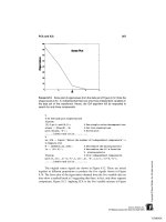
Figure 12.1 shows an x-ray image of the spine image with its associated density
histogram. Figure 12.1 also shows the binary image obtained by applying a
threshold at a specific point on the histogram. When RGB color images are
being analyzed, intensity histograms can be obtained from all three color planes
and different thresholds established for each color plane with the aid of the
corresponding histogram.
Intensity histograms can be very helpful in selecting threshold levels, not
only for the original image, but for images produced by various segmentation
algorithms described later. Intensity histograms can also be useful in evaluating
the efficacy of different processing schemes: as the separation between struc-
tures improves, histogram peaks should become more distinctive. This relation-
ship between separation and histogram shape is demonstrated in Figures 12.2
and, more dramatically, in Figures 12.3 and 12.4.
TLFeBOOK
Image Segmentation 345
F
IGURE
12.1 An image of bone marrow, upper left, and its associated intensity
histogram, lower plot. The upper right image is obtained by thresholding the origi-
nal image at a value corresponding to the vertical line on the histogram plot.
(Original image from the MATLAB Image Processing Toolbox. Copyright 1993–
2003, The Math Works, Inc. Reprinted with permission.)
Intensity histograms contain no information on position, yet it is spatial
information that is of prime importance in problems of segmentation, so some
strategies have been developed for determining threshold(s) from the histogram
(Sonka et al. 1993). If the intensity histogram is, or can be assumed as, bimodal
(or multi-modal), a common strategy is to search for low points, or minima, in
the histogram. This is the strategy used in Figure 12.1, where the threshold was
set at 0.34, the intensity value at which the histogram shows an approximate
minimum. Such points represent the fewest number of pixels and should pro-

duce minimal classification errors; however, the histogram minima are often
difficult to determine due to variability.
TLFeBOOK
346 Chapter 12
F
IGURE
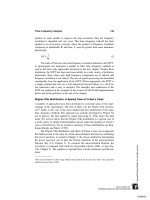
12.2 Image of bloods cells with (upper) and without (lower) intermediate
boundaries removed. The associated histograms (right side) show improved sep-
arability when the boundaries are eliminated. The code that generated these im-
ages is given in Example 12.1. (Original image reprinted with permission from
the Image Processing Handbook 2nd edition. Copyright CRC Press, Boca Raton,
Florida.)
An approach to improve the determination of histogram minima is based
on the observation that many boundary points carry values intermediate to the
values on either side of the boundary. These intermediate values will be associ-
ated with the region between the actual boundary values and may mask the
optimal threshold value. However, these intermediate points also have the high-
est gradient, and it should be possible to identify them using a gradient-sensitive
filter, such as the Sobel or Canny filter. After these boundary points are identi-
fied, they can be eliminated from the image, and a new histogram is computed
with a distribution that is possibly more definitive. This strategy is used in
TLFeBOOK
Image Segmentation 347
F
IGURE
12.3 Thresholded blood cell images. Optimal thresholds were applied to
the blood cell images in Figure 12.2 with (left) and without (right) boundaries pixel
masked. Fewer inappropriate pixels are seen in the right image.
Example 12.1, and Figure 12.2 shows images and associated histograms before
and after removal of boundary points as identified using Canny filtering. The

reduction in the number of intermediate points can be seen in the middle of the
histogram (around 0.45). As shown in Figure 12.3, this leads to slightly better
segmentation of the blood cells.
Another histogram-based strategy that can be used if the distribution is
bimodal is to assume that each mode is the result of a unimodal, Gaussian
distribution. An estimate is then made of the underlying distributions, and the
point at which the two estimated distributions intersect should provide the opti-
mal threshold. The principal problem with this approach is that the distributions
are unlikely to be truly Gaussian.
A threshold strategy that does not use the histogram is based on the con-
cept of minimizing the variance between presumed foreground and background
elements. Although the method assumes two different gray levels, it works well
even when the distribution is not bimodal (Sonka et al., 1993). The approach
uses an iterative process to find a threshold that minimizes the variance between
the intensity values on either side of the threshold level (Outso’s method). This
approach is implemented using the MATLAB routine
grayslice
(see Example
12.1).
A pixel-based technique that provides a segment boundary directly is con-
tour mapping. Contours are lines of equal intensity, and in a continuous image
they are necessarily continuous: they cannot end within the image, although
TLFeBOOK
348 Chapter 12
F
IGURE
12.4 Contour maps drawn from the blood cell image of Figures 12.2 and
12.3. The right image was pre-filtered with a Gaussian lowpass filter (alpha = 3)
before the contour lines were drawn. The contour values were set manually to
provide good images.

they can branch or loop back on themselves. In digital images, these same prop-
erties exist but the value of any given contour line will not generally equal the
values of the pixels it traverses. Rather, it usually reflects values intermediate
between adjacent pixels. To use contour mapping to identify image structures
requires accurate setting of the contour levels, and this carries the same burdens
as thresholding. Nonetheless, contour maps do provide boundaries directly, and,
if subpixel interpolation is used in establishing the contour position, they may
be spatially more accurate. Contour maps are easy to implement in MATLAB,
as shown in the next section on MATLAB Implementation. Figure 12.4 shows
contours maps for the blood cell images shown in Figure 12.2. The right image
was pre-filtered with a Gaussian lowpass filter which reduces noise slightly and
improves the resultant contour image.
Pixel-based approaches can lead to serious errors, even when the average
intensities of the various segments are clearly different, due to noise-induced
intensity variation within the structure. Such variation could be acquired during
image acquisition, but could also be inherent in the structure itself. Figure 12.5
shows two regions with quite different average intensities. Even with optimal
threshold selection, many inappropriate pixels are found in both segments due
to intensity variations within the segments Fig 12.3 (right). Techniques for im-
proving separation in such images are explored in the sections on continuity-
based approaches.
TLFeBOOK
Image Segmentation 349
F
IGURE
12.5 An image with two regions having different average gray levels.
The two regions are clearly distinguishable; however, using thresholding alone, it
is not possible to completely separate the two regions because of noise.
MATLAB Implementation
Some of the routines for implementing pixel-based operations such as

im2bw
and
grayslice
have been described in preceding chapters. The image intensity
histogram routine is produced by
imhist
without the output arguments:
[counts, x] = imhist(I, N);
where
counts
is the histogram value at a given
x
,
I
is the image, and
N
is an
optional argument specifying the number of histogram bins (the default is 255).
As mentioned above,
imhist
is usually invoked without the output arguments,
count
and
x
, to produce a plot directly.
The rescale routine is:
I_rescale = imscale(I, [low high], [bottom top], gamma);
where
I_rescale
is the rescaled output image,

I
is the input image. The range
between
low
and
high
in the input image is rescaled to be between bottom and
top in the output image.
Several pixel-based techniques are presented in Example 12.1.
Example 12.1 An example of segmentation using pixel-based methods.
Load the image of blood cells, and display along with the intensity histogram.
Remove the edge pixels from the image and display the histogram of this modi-
TLFeBOOK
350 Chapter 12
F
IGURE
12.6A Histogram of the image shown in Figure 12.3 before (upper) and
after (lower) lowpass filtering. Before filtering the two regions overlap to such an
extend that they cannot be identified. After lowpass filtering, the two regions are
evident, and the boundary found by minimum variance is shown. The application
of this boundary to the filtered image results in perfect separation as shown in
Figure 12.4B.
fied image. Determine thresholds using the minimal variance iterative technique
described above, and apply this approach to threshold both images. Display the
resultant thresholded images.
Solution To remove the edge boundaries, first identify these boundaries
using an edge detection scheme. While any of the edge detection filters de-
scribed previously can be used, this application will use the Canny filter as it is
most robust to noise. This filter is implemented as an option of MATLAB’s
edge

routine, which produces a binary image of the boundaries. This binary
image will be converted to a boundary mask by inverting the image using
imcomplement
. After inversion, the edge pixels will be zero while all other
pixels will be one. Multiplying the original image by the boundary mask will
produce an image in which the boundary points are removed (i.e., set to zero,
or black). All the images involved in this process, including the original image,
will then be plotted.
TLFeBOOK
Image Segmentation 351
F
IGURE
12.6B Left side: The same image shown in Figure 12.5 after lowpass
filtering. Right side: This filtered image can now be perfectly separated by thresh-
olding.
% Example 12.1 and Figure 12.2 and Figure 12.3
% Lowpass filter blood cell image, then display histograms
% before and after edge point removal.
% Applies “optimal” threshold routine to both original and
% “masked” images and display the results
%
input image and convert to double
h = fspecial(‘gaussian’,12,2); % Construct gaussian
% filter
I_f = imfilter(I,h,‘replicate’); % Filter image
%
I_edge = edge(I_f,‘canny’,.3); % To remove edge
I_rem = I_f .* imcomplement(I_edge); % points, find edge,
% complement and use
% as mask

%
subplot(2,2,1); imshow(I_f); % Display images and
% histograms
title(‘Original Figure’);
subplot(2,2,2); imhist(I_f); axis([0 1 0 1000]);
title(‘Filtered histogram’);
subplot(2,2,3); imshow(I_rem);
title(‘Edge Removed’);
subplot(2,2,4); imhist(I_rem); axis([0 1 0 1000]);
title(‘Edge Removed histogram’);
TLFeBOOK
352 Chapter 12
%
figure; % Threshold and
% display images
t1 = graythresh(I); % Use minimum variance
% thresholds
t2 = graythresh(I_f);
subplot(1,2,1); imshow(im2bw(I,t1));
title(‘Threshold Original Image’);
subplot(1,2,2); imshow(im2bw(I_f,t2));
title(‘Threshold Masked Image’);
The results have been shown previously in Figures 12.2 and 12.3, and the
improvement in the histogram and threshold separation has been mentioned.
While the change in the histogram is fairly small (Figure 12.2), it does lead to
a reduction in artifacts in the thresholded image, as shown in Figure 12.3. This
small improvement could be quite significant in some applications. Methods
for removing the small remaining artifacts will be described in the section on
morphological operations.
CONTINUITY-BASED METHODS

These approaches look for similarities or consistency in the search for structural
units. As demonstrated in the examples below, these approaches can be very
effective in segmentation tasks, but they all suffer from a lack of edge definition.
This is because they are based on neighborhood operations and these tend to
blur edge regions, as edge pixels are combined with structural segment pixels.
The larger the neighborhood used, the more poorly edges will be defined. Unfor-
tunately, increasing neighborhood size usually improves the power of any given
continuity-based operation, setting up a compromise between identification abil-
ity and edge definition. One easy technique that is based on continuity is low-
pass filtering. Since a lowpass filter is a sliding neighborhood operation that
takes a weighted average over a region, it enhances consistent characteristics.
Figure 12.6A shows histograms of the image in Figure 12.5 before and after
filtering with a Gaussian lowpass filter (alpha = 1.5). Note the substantial im-
provement in separability suggested by the associated histograms. Applying a
threshold to the filtered image results in perfectly isolated segments as shown
in Figure 12.6B. The thresholded images in both Figures 12.5 and 12.4B used
the same minimum variance technique to set the threshold, yet the improvement
brought about by simple lowpass filtering is remarkable.
Image features related to texture can be particularly useful in segmenta-
tion. Figure 12.7 shows three regions that have approximately the same average
intensity values, but are readily distinguished visually because of differences in
texture. Several neighborhood-based operations can be used to distinguish tex-
TLFeBOOK
Image Segmentation 353
tures: the small segment Fourier transform, local variance (or standard devia-
tion), the Laplacian operator, the range operator (the difference between maxi-
mum and minimum pixel values in the neighborhood), the Hurst operator
(maximum difference as a function of pixel separation), and the Haralick opera-
tor (a measure of distance moment). Many of these approaches are either di-
rectly supported in MATLAB, or can be implement using the

nlfilter
routine
described in Chapter 10.
MATLAB Implementation
Example 12.2 attempts to separate the three regions shown in Figure 12.7 by
applying one of these operators to convert the texture pattern to a difference in
intensity that can then be separated using thresholding.
Example 12.2 Separate out the three segments in Figure 12.7 that differ
only in texture. Use one of the texture operators described above and demon-
strate the improvement in separability through histogram plots. Determine ap-
propriate threshold levels for the three segments from the histogram plot.
F
IGURE
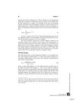
12.7 An image containing three regions having approximately the same
intensity, but different textures. While these areas can be distinguished visually,
separation based on intensity or edges will surely fail. (Note the single peak in
the intensity histogram in Figure 12.9–upper plot.)
TLFeBOOK
354 Chapter 12
Solution Use the nonlinear range filter to convert the textural patterns
into differences in intensity. The range operator is a sliding neighborhood proce-
dure that takes the difference between the maximum and minimum pixel value
with a neighborhood. Implement this operation using MATLAB’s
nlfilter
routine with a 7-by-7 neighborhood.
% Example 12.2 Figures 12.8, 12.9, and 12.10
% Load imag e ‘texture3. tif’ which contains thre e regions having
% the same average intensities, but different textural patterns.
% Apply the “range” nonlinear operator using ‘nlfilter’
% Plot original and range histograms and filtered image

%
clear all; close all;
[I] = imread(‘texture3.tif’); % Load image and
I = im2double(I); % Convert to double
%
range = inline(‘max(max(x))— % Define Range function
min (min(x))’);
I_f = nlfilter(I,[7 7], range); % Compute local range
I_f = mat2gray(I_f); % Rescale intensities
F
IGURE
12.8 The texture pattern shown in Figure 12.7 after application of the
nonlinear range operation. This operator converts the textural properties in the
original figure into a difference in intensities. The three regions are now clearly
visible as intensity differences and can be isolated using thresholding.
TLFeBOOK
Image Segmentation 355
F
IGURE
12.9 Histogram of original texture pattern before (upper) and after non-
linear filtering using the range operator (lower). After filtering, the three intensity
regions are clearly seen. The thresholds used to isolate the three segments are
indicated.
%
imshow(I_f); % Display results
title(‘“Range” Image’);
figure;
subplot(2,1,1); imhist(I); % Display both histograms
title(‘Original Histogram’)
subplot(2,1,2); imhist(I_f);

title(‘“Range” Histogram’);
figure;
subplot(1,3,1); imshow(im2bw % Display three segments
(I_f,.22));
subplot(1,3,2); imshow(islice % Uses ’islice’ (see below)
(I_f,.22,.54));
subplot(1,3,3); imshow(im2bw(I_f,.54));
TLFeBOOK
356 Chapter 12
The image produced by the range filter is shown in Figure 12.8, and a
clear distinction in intensity level can now be seen between the three regions.
This is also demonstrated in the histogram plots of Figure 12.9. The histogram
of the original figure (upper plot) shows a single Gaussian-like distribution with
no evidence of the three patterns.* After filtering, the three patterns emerge as
three distinct distributions. Using this distribution, two thresholds were chosen
at minima between the distributions (at 0.22 and 0.54: the solid vertical lines in
Figure 12.9) and the three segments isolated based on these thresholds. The two
end patterns could be isolated using
im2bw
, but the center pattern used a special
routine,
islice
. This routine sets pixels to one whose values fall between an
upper and lower boundary; if the pixel has values above or below these bound-
aries, it is set to zero. (This routine is on the disk.) The three fairly well sepa-
rated regions are shown in Figure 12.10. A few artifacts remain in the isolated
images, and subsequent methods can be used to eliminate or reduce these erro-
neous pixels.
Occasionally, segments will have similar intensities and textural proper-
ties, except that the texture differs in orientation. Such patterns can be distin-

guished using a variety of filters that have orientation-specific properties. The
local Fourier transform can also be used to distinguish orientation. Figure 12.11
shows a pattern with texture regions that are different only in terms of their
orientation. In this figure, also given in Example 12.3, orientation was identified
F
IGURE
12.10 Isolated regions of the texture pattern in Figure 12.7. Although
there are some artifact, the segmentation is quite good considering the original
image. Methods for reducing the small artifacts will be given in the section on
edge detection.
*In fact, the distribution is Gaussian since the image patterns were generated by filtering an array
filled with Gaussianly distributed numbers generated by
randn
.
TLFeBOOK
Image Segmentation 357
F
IGURE
12.11 Textural pattern used in Example 12.3. The horizontal and vertical
patterns have the same textural characteristics except for their orientation. As in
Figure 12.7, the three patterns have the same average intensity.
by application of a direction operator that operates only in the horizontal direc-
tion. This is followed by a lowpass filter to improve separability. The intensity
histograms in Figure 12.12 shown at the end of the example demonstrate the
intensity separations achieved by the directional range operator and the improve-
ment provided by the lowpass filter. The different regions are then isolated using
threshold techniques.
Example 12.3 Isolate segments from a texture pattern that includes two
patterns with the same textural characteristics except for orientation. Note that
the approach used in Example 12.2 will fail: the similarity in the statistical

properties of the vertical and horizontal patterns will give rise to similar intensi-
ties following a range operation.
Solution Apply a filter that has directional sensitivity. A Sobel or Prewitt
filter could be used, followed by the range or similar operator, or the operations
could be done in a single step by using a directional range operator. The choice
made in this example is to use a horizontal range operator implemented with
nlfilter
. This is followed by a lowpass filter (Gaussian, alpha = 4) to improve
separation by removing intensity variation. Two segments are then isolated us-
ing standard thresholding. In this example, the third segment was constructed
TLFeBOOK
358 Chapter 12
F
IGURE
12.12 Images produced by application of a direction range operator ap-
plied to the image in Figure 12.11 before (upper) and after (lower) lowpass filter-
ing. The histograms demonstrate the improved separability of the filter image
showing deeper minima in the filtered histogram.
by applying a logical operation to the other two segments. Alternatively, the
islice
routine could have been used as in Example 12.2.
% Example 12.3 and Figures 12.11, 12.12, and 12.13
% Analysis of texture pattern having similar textural
% characteristics but with different orientations. Use a
% direction-specific filter.
%
clear all; close all;
I = imread(‘texture4.tif’); % Load “orientation” texture
I = im2double(I); % Convert to double
TLFeBOOK

Image Segmentation 359
F
IGURE
12.13 Isolated segments produced by thresholding the lowpass filtered
image in Figure 12.12. The rightmost segment was found by applying logical op-
erations to the other two images.
%
% Define filters and functions: I-D range function
range = inline(‘max(x)—min(x)’);
h_lp = fspecial (‘gaussian’, 20, 4);
%
% Directional nonlinear filter
I_nl = nlfilter(I, [9 1], range);
I_h = imfilter(I_nl*2, h_lp); % Average (lowpass filter)
%
subplot(2,2,1); imshow % Display image and histogram
(I_nl*2); % before lowpass filtering
title(‘Modified Image’); % and after lowpass filtering
subplot(2,2,2); imhist(I_nl);
title(‘Histogram’);
subplot(2,2,3); imshow(I_h*2); % Display modified image
title(‘Modified Image’);
subplot(2,2,4); imhist(I_h);
title(‘Histogram’);
%
figure;
BW1 = im2bw(I_h,.08); % Threshold to isolate segments
BW2 = ϳim2bw(I_h,.29);
BW3 = ϳ(BW1 & BW2); % Find third image from other
% two

subplot(1,3,1); imshow(BW1); % Display segments
subplot(1,3,2); imshow(BW2);
subplot(1,3,3); imshow(BW3);
TLFeBOOK
360 Chapter 12
The image produced by the horizontal range operator with, and without,
lowpass filtering is shown in Figure 12.12. Note the improvement in separation
produced by the lowpass filtering as indicated by a better defined histogram.
The thresholded images are shown in Figure 12.13. As in Example 12.2, the
separation is not perfect, but is quite good considering the challenges posed by
the original image.
Multi-Thresholding
The results of several different segmentation approaches can be combined either
by adding the images together or, more commonly, by first thresholding the
images into separate binary images and then combining them using logical oper-
ations. Either the AND or OR operator would be used depending on the charac-
teristics of each segmentation procedure. If each procedure identified all of the
segments, but also included non-desired areas, the AND operator could be used
to reduce artifacts. An example of the use of the AND operation was found
in Example 12.3 where one segment was found using the inverse of a logical
AND of the other two segments. Alternatively, if each procedure identified
some portion of the segment(s), then the OR operator could be used to com-
bine the various portions. This approach is illustrated in Example 12.4 where
first two, then three, thresholded images are combined to improve segment iden-
tification. The structure of interest is a cell which is shown on a gray back-
ground. Threshold levels above and below the gray background are combined
(after one is inverted) to provide improved isolation. Including a third binary
image obtained by thresholding a texture image further improves the identifica-
tion.
Example 12.4 Isolate the cell structures from the image of a cell shown

in Figure 12.14.
Solution Since the cell is projected against a gray background it is possi-
ble to isolate some portions of the cell by thresholding above and below the
background level. After inversion of the lower threshold image (the one that is
below the background level), the images are combined using a logical OR. Since
the cell also shows some textural features, a texture image is constructed by
taking the regional standard deviation (Figure 12.14). After thresholding, this
texture-based image is also combined with the other two images.
% Example 12.4 and Figures 12.14 and 12.15
% Analysis of the image of a cell using texture and intensity
% information then combining the resultant binary images
% with a logical OR operation.
clear all; close all;
I = imread(‘cell.tif’); % Load “orientation” texture
TLFeBOOK
Image Segmentation 361
F
IGURE
12.14 Image of cells (left) on a gray background. The textural image
(right) was created based on local variance (standard deviation) and shows
somewhat more definition. (Cancer cell from rat prostate, courtesy of Alan W.
Partin, M.D., Ph.D., Johns Hopkins University School of Medicine.)
I = im2double(I); % Convert to double
%
h = fspecial(‘gaussian’, 20, 2); % Gaussian lowpass filter
%
subplot(1,2,1); imshow(I); % Display original image
title(‘Original Image’);
I_std = (nlfilter(I,[3 3], % Texture operation
’std2’))*6;

I_lp = imfilter(I_std, h); % Average (lowpass filter)
%
subplot(1,2,2); imshow(I_lp*2); % Display texture image
title(‘Filtered image’);
%
figure;
BW_th = im2bw(I,.5); % Threshold image
BW_thc = ϳim2bw(I,.42); % and its complement
BW_std = im2bw(I_std,.2); % Threshold texture image
BW1 = BW_th * BW_thc; % Combine two thresholded
% images
BW2 = BW_std * BW_th * BW_thc; % Combine all three images
subplot(2,2,1); imshow(BW_th); % Display thresholded and
subplot(2,2,2); imshow(BW_thc); % combined images
subplot(2,2,3); imshow(BW1);
TLFeBOOK
362 Chapter 12
F
IGURE
12.15 Isolated portions of the cells shown in Figure 12.14. The upper
images were created by thresholding the intensity. The lower left image is a com-
bination (logical OR) of the upper images and the lower right image adds a
thresholded texture-based image.
The original and texture images are shown in Figure 12.14. Note that the
texture image has been scaled up, first by a factor of six, then by an additional
factor of two, to bring it within a nominal image range. The intensity thresh-
olded images are shown in Figure 12.15 (upper images; the upper right image
has been inverted). These images are combined in the lower left image. The
lower right image shows the combination of both intensity-based images with
the thresholded texture image. This method of combining images can be ex-

tended to any number of different segmentation approaches.
MORPHOLOGICAL OPERATIONS
Morphological operations have to do with processing shapes. In this sense they
are continuity-based techniques, but in some applications they also operate on
TLFeBOOK
Image Segmentation 363
edges, making them useful in edge-based approaches as well. In fact, morpho-
logical operations have many image processing applications in addition to seg-
mentation, and they are well represented and supported in the MATLAB Image
Processing Toolbox.
The two most common morphological operations are dilation and erosion.
In dilation the rich get richer and in erosion the poor get poorer. Specifically,
in dilation, the center or active pixel is set to the maximum of its neighbors,
and in erosion it is set to the minimum of its neighbors. Since these operations
are often performed on binary images, dilation tends to expand edges, borders,
or regions, while erosion tends to decrease or even eliminate small regions.
Obviously, the size and shape of the neighborhood used will have a very strong
influence on the effect produced by either operation.
The two processes can be done in tandem, over the same area. Since both
erosion and dilation are nonlinear operations, they are not invertible transforma-
tions; that is, one followed by the other will not generally result in the original
image. If erosion is followed by dilation, the operation is termed opening.Ifthe
image is binary, this combined operation will tend to remove small objects
without changing the shape and size of larger objects. Basically, the initial ero-
sion tends to reduce all objects, but some of the smaller objects will disappear
altogether. The subsequent dilation will restore those objects that were not elimi-
nated by erosion. If the order is reversed and dilation is performed first followed
by erosion, the combined process is called closing. Closing connects objects
that are close to each other, tends to fill up small holes, and smooths an object’s
outline by filling small gaps. As with the more fundamental operations of dila-

tion and erosion, the size of objects removed by opening or filled by closing
depends on the size and shape of the neighborhood that is selected.
An example of the opening operation is shown in Figure 12.16 including
the erosion and dilation steps. This is applied to the blood cell image after
thresholding, the same image shown in Figure 12.3 (left side). Since we wish
to eliminate black artifacts in the background, we first invert the image as shown
in Figure 12.16. As can be seen in the final, opened image, there is a reduction
in the number of artifacts seen in the background, but there is also now a gap
created in one of the cell walls. The opening operation would be more effective
on the image in which intermediate values were masked out (Figure 12.3, right
side), and this is given as a problem at the end of the chapter.
Figure 12.17 shows an example of closing applied to the same blood cell
image. Again the operation was performed on the inverted image. This operation
tends to fill the gaps in the center of the cells; but it also has filled in gaps
between the cells. A much more effective approach to filling holes is to use the
imfill
routine described in the section on MATLAB implementation.
Other MATLAB morphological routines provide local maxima and min-
ima, and allows for manipulating the image’s maxima and minima, which im-
plement various fill-in effects.
TLFeBOOK
364 Chapter 12
F
IGURE
12.16 Example of the opening operation to remove small artifacts. Note
that the final image has fewer background spots, but now one of the cells has a
gap in the wall.
MATLAB Implementation
The erosion and dilation could be implemented using the nonlinear filter routine
nlfilter

, although this routine limits the shape of the neighborhood to a rect-
angle. The MATLAB routines
imdilate
and
imerode
provide for a variety of
neighborhood shapes and are much faster than
nlfilter
. As mentioned above,
opening consists of erosion followed by dilation and closing is the reverse.
MATLAB also provide routines for implementing these two operations in one
statement.
To specify the neighborhood used by all of these routines, MATLAB uses
a structuring element.* A structuring element can be defined by a binary array,
where the ones represent the neighborhood and the zeros are irrelevant. This
allows for easy specification of neighborhoods that are nonrectangular, indeed
that can have any arbitrary shape. In addition, MATLAB makes a number of
popular shapes directly available, just as the
fspecial
routine makes a number
*Not to be confused with a similar term, structural unit, used in the beginning of this chapter. A
structural unit is the object of interest in the image.
TLFeBOOK
Image Segmentation 365
F
IGURE
12.17 Example of closing to fill gaps. In the closed image, some of the
cells are now filled, but some of the gaps between cells have been erroneously
filled in.
of popular two-dimensional filter functions available. The routine to specify the

structuring element is
strel
and is called as:
structure = strel(shape, NH, arg);
where
shape
is the type of shape desired,
NH
usually specifies the size of the
neighborhood, and
arg
and an argument, frequently optional, that depends on
shape
.If
shape
is
‘arbitrary’
, or simply omitted, then
NH
is an array that
specifies the neighborhood in terms of ones as described above. Prepackaged
shapes include:
‘disk’
a circle of radius
NH
(in pixels)
‘line’
a line of length
NH
and angle

arg
in degrees
‘rectangle’
a rectangle where
NH
is a two element vector specifying rows and col-
umns
‘diamond’
a diamond where
NH
is the distance from the center to each corner
‘square’
a square with linear dimensions
NH
TLFeBOOK
366 Chapter 12
For many of these shapes, the routine
strel
produces a decomposed
structure that runs significantly faster.
Based on the structure, the statements for dilation, erosion, opening, and
closing are:
I1 = imdilate(I, structure);
I1 = imerode(I, structure);
I1 = imopen(I, structuure);
I1 = imclose(I, structure);
where
I1
is the output image,
I

is the input image and
structure
is the neigh-
borhood specification given by
strel
, as described above. In all cases,
struc-
ture
can be replaced by an array specifying the neighborhood as ones, bypass-
ing the
strel
routine. In addition,
imdilate
and
imerode
have optional
arguments that provide packing and unpacking of the binary input or output
images.
Example 12.5 Apply opening and closing to the thresholded blood cell
images of Figure 12–3 in an effort to remove small background artifacts and to
fill holes. Use a circular structure with a diameter of four pixels.
% Example 12.5 and Figures 12.16 and 12.17
% Demonstration of morphological opening to eliminate small
% artifacts and of morphological closing to fill gaps
% These operations will be applied to the thresholded blood cell
% images of Figure 12.3 (left image).
% Uses a circular or disk shaped structure 4 pixels in diameter
%
clear all; close all;
I = imread(‘blood1.tif’); % Get image and threshold

I = im2double(I);
BW = ϳim2bw(I,thresh(I));
%
SE = strel(‘disk’,4); % Define structure: disk of radius
% 4 pixels
BW1= imerode(BW,SE); % Opening operation: erode
BW2 = imdilate(BW1,SE); % image first, then dilate
%
display images
%
BW3= imdilate(BW,SE); % Closing operation, dilate image
BW4 = imerode(BW3,SE); % first then erode
%
display images
TLFeBOOK
Image Segmentation 367
This example produced the images in Figures 12.15 and 12.16.
Example 12.6 Apply an opening operation to remove the dark patches
seen in the thresholded cell image of Figure 12.15.
% Figures 12.6 and 12.18
% Use opening to remove the dark patches in the thresholded cell
% image of Figure 12.15
%
close all; clear all;
%
SE = strel(‘square’,5); % Define closing structure:
% square 5 pixels on a side
load fig12_15; % Get data of Figure 12.15 (BW2)
BW1= ϳimopen(ϳBW2,SE); % Opening operation
Display images

The result of this operation is shown in Figure 12.18. In this case, the
closing operation is able to remove completely the dark patches in the center of
the cell image. A 5-by-5 pixel square structural element was used. The size (and
shape) of the structural element controlled the size of artifact removed, and no
attempt was made to optimize its shape. The size was set here as the minimum
that would still remove all of the dark patches. The opening operation in this
example used the single statement
imopen
. Again, the opening operation oper-
ates on activated (i.e., white pixels), so to remove dark artifacts it is necessary
to invert the image (using the logical NOT operator, ϳ) before performing the
opening operation. The opened image is then inverted again before display.
F
IGURE
12.18 Application of the open operation to remove the dark patches in
the binary cell image in Figure 12.15 (lower right). Using a 5 by 5 square struc-
tural element resulted in eliminating all of the dark patches.
TLFeBOOK
368 Chapter 12
MATLAB morphology routines also allow for manipulation of maxima
and minima in an image. This is useful for identifying objects, and for filling.
Of the many other morphological operations supported by MATLAB, only the
imfill
operation will be described here. This operation begins at a designated
pixel and changes connected background pixels (0’s) to foreground pixels (1’s),
stopping only when a boundary is reached. For grayscale images,
imfill
brings
the intensity levels of the dark areas that are surrounded by lighter areas up to
the same intensity level as surrounding pixels. (In effect,

imfill
removes re-
gional minima that are not connected to the image border.) The initial pixel can
be supplied to the routine or obtained interactively. Connectivity can be defined
as either four connected or eight connected. In four connectivity, only the four
pixels bordering the four edges of the pixel are considered, while in eight con-
nectivity all pixel that touch, including those that touch only at the corners, are
considered connected.
The basic
imfill
statement is:
I_out = imfill(I, [r c], con);
where
I
is the input image,
I_out
is the output image,
[r c]
is a two-element
vector specifying the beginning point, and
con
is an optional argument that is
set to 8 for eight connectivity (four connectivity is the default). (See the help
file to use
imfill
interactively.) A special option of
imfill
is available specifi-
cally for filling holes. If the image is binary, a hole is a set of background pixels
that cannot be reached by filling in the background from the edge of the image.

If the image is an intensity image, a hole is an area of dark pixels surrounded
by lighter pixels. To invoke this option, the argument following the input image
should be
holes
. Figure 12.19 shows the operation performed on the blood cell
image by the statement:
I_out = imfill(I, ‘holes’);
EDGE-BASED SEGMENTATION
Historically, edge-based methods were the first set of tools developed for seg-
mentation. To move from edges to segments, it is necessary to group edges into
chains that correspond to the sides of structural units, i.e., the structural bound-
aries. Approaches vary in how much prior information they use, that is, how
much is used of what is known about the possible shape. False edges and missed
edges are two of the more obvious, and more common, problems associated
with this approach.
The first step in edge-based methods is to identify edges which then be-
come candidates for boundaries. Some of the filters presented in Chapter 11
TLFeBOOK