Data Analysis Machine Learning and Applications Episode 1 Part 3 docx

Computer Assisted Classification of Brain Tumors
Norbert Röhrl
1
, José R. Iglesias-Rozas
2
and Galia Weidl
1
1
Institut für Analysis, Dynamik und Modellierung, Universität Stuttgart
Pfaffenwaldring 57, 70569 Stuttgart, Germany

2
Katharinenhospital, Institut für Pathologie, Neuropathologie
Kriegsbergstr. 60, 70174 Stuttgart, Germany

Abstract. The histological grade of a brain tumor is an important indicator for choosing the
treatment after resection. To facilitate objectivity and reproducibility, Iglesias et al. (1986)
proposed to use a standardized protocol of 50 histological features in the grading process.
We tested the ability of Support Vector Machines (SVM), Learning Vector Quantization
(LVQ) and Supervised Relevance Neural Gas (SRNG) to predict the correct grades of the
794 astrocytomas in our database. Furthermore, we discuss the stability of the procedure with
respect to errors and propose a different parametrization of the metric in the SRNG algorithm
to avoid the introduction of unnecessary boundaries in the parameter space.
1 Introduction
Although the histological grade has been recognized as one of the most powerful
predictors of the biological behavior of tumors and significantly affects the manage-
ment of patients, it suffers from low inter- and intraobserver reproducibility due to
the subjectivity inherent to visual observation. The common procedure for grading
is that a pathologist looks at the biopsy under a microscope and then classifies the
tumor on a scale of 4 grades from I to IV (see Fig. 1). The grades roughly correspond
to survival times: a patient with a grade I tumor can survive 10 or more years, while

a patient with a grade IV tumor dies with high probability within 15 month. Iglesias
et al. (1986) proposed to use a standardized protocol of 50 histological features in
addition to make grading of tumors reproducible and to provide data for statistical
analysis and classification.
The presence of these 50 histological features (Fig. 2) was rated in 4 categories
from 0 (not present) to 3 (abundant) by visual inspection of the sections under a
microscope. The type of astrocytoma was then determined by an expert and the cor-
responding histological grade between I and IV is assigned.
56 Norbert Röhrl, José R. Iglesias-Rozas and Galia Weidl
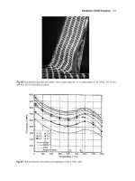
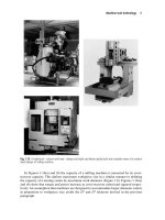
Fig. 1. Pictures of biopsies under a microscope. The larger picture is healthy brain tissue
with visible neurons. The small pictures are tumors of increasing grade from left top to right
bottom. Note the increasing number of cell nuclei and increasing disorder.
+ ++ +++
Fig. 2. One the 50 histological features: Concentric arrangement. The tumor cells build con-
centric formations with different diameters.
2 Algorithms
We chose LVQ (Kohonen (1995)), SRNG (Villmann et al. (2002)) and SVM (Vap-
nik (1995)) to classify this high dimensional data set, because the generalization
error (expectation value of misclassification) of these algorithms does not depend on
the dimension of the feature space (Barlett and Mendelson (2002), Crammer et al.
(2003), Hammer et al. (2005)).
For the computations we used the original LVQ-PAK (Kohonen et al. (1992)),
LIBSVM (Chan and Lin (2001)) and our own implementation of SRNG, since to our
knowledge there exists no freely available package. Moreover for obtaining our best
results, we had to deviate in some respects from the description given in the original
article (Villmann et al. (2002)). In order to be able to discuss our modification we
briefly formulate the original algorithm.
2.1 SRNG
Let the feature space be R
n

and fix a discrete set of labels Y , a training set T ⊆
R
n
×Y and a prototype set C ⊆R
n
×Y .
The distance in feature space is defined to be
Computer Assisted Classification of Brain Tumors 57
d
O
(x, ˜x)=
n

i=1
O
i
|x
i
− ˜x
i
|
2
.
with parameters O =(O
1
, ,O
n
) ∈R
n
, O

i
≥0and

O
i
= 1. Given a sample (x,y) ∈
T,wedefine denote its distance to the closest prototype with a different label by
d
−
O
(x,y),
d
−
O
(x,y) := min{d(x, ˜x)|( ˜x, ˜y) ∈C, y ≡ ˜y}.
We denote the set of all prototypes with label y by
W
y
:= {( ˜x, y) ∈C}
and enumerate its elements ( ˜x, ˜y) according to their distance to (x,y)
rg
(x,y)
( ˜x, ˜y) :=


{( ˆx, ˆy) ∈W
y
|d(ˆx,x) < d( ˜x,x)}



.
Then the loss of a single sample (x,y) ∈T is given by
L
C,O
(x,y) :=
1
c

( ˜x,y)∈W
y
exp

J
−1
rg
(x,y)
( ˜x, y)

sgd

d
O
(x, ˜x) −d
−
O
d
O
(x, ˜x)+d
−
O


,
where J is the neighborhood range, sgd =(1 +exp(−x))
−1
the sigmoid function and
c =
|W
y
|−1

n=0
e
J
−1
n
a normalization constant. The actual SRNG algorithm now minimizes the total loss
of the training set T ⊂ X
L
C,O
(T)=

(x,y)∈T
L
C,O
(x,y) (1)
by stochastic gradient descent with respect to the prototypes C and the parameters of
the metric O, while letting the neighborhood range J approach zero. This in particular
reduces the dependence on the initial choice of the prototypes, which is a common
problem with LVQ.
Stochastic gradient descent means here, that we compute the gradients 

C
L and

O
L of the loss function L
C,O
(x,y) of a single randomly chosen element (x,y) of the
training set and replace C by C −H
C

C
L and O by O −H
O

O
L with small learning
rates H
C
> 10H
O
> 0. The different magnitude of the learning rates is important, be-
cause classification is primarily done using the prototypes. If the metric is allowed to
change too quickly, the algorithm will in most cases end in a suboptimal minimum.
58 Norbert Röhrl, José R. Iglesias-Rozas and Galia Weidl
2.2 Modified SRNG
In our early experiments and while tuning SRNG for our task, we found two prob-
lems with the distance used in feature space.
The straight forward parametrization of the metric comes at the price of intro-
ducing the boundaries O
i

≥ 0, which in practice are often hit too early and knock
out the corresponding feature. Also, artificially setting negative O
i
to zero does slow
down the convergence process.
The other point is, that by choosing different learning rates H
C
and H
O
for proto-
types and metric parameters, we are no longer using the gradient of the given loss
function (1), which can also be problematic in the convergence process.
We propose using the following metric for measuring distance in feature space
d
O
(x, ˜x)=
n

i=1
e
rO
i
|x
i
− ˜x
i
|
2
,
where the dependence on O

i
is exponential and we introduce a scaling factor r > 0.
This definition avoids explicit boundaries for O
i
and r allows to adjust the rate of
change of the distance function relative to the prototypes. Hence this parametriza-
tion enables us to minimize the loss function by stochastic gradient descent without
treating prototypes and metric parameters separately.
3 Results
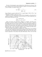
To test the prediction performance of the algorithms (Table 3), we divided the 794
cases (grade I: 156, grade II: 362, grade III: 238, grade 4: 38) into 10 subsets of equal
size and grade distribution for cross validation.
For SVM we used a RBF kernel and let LIBSVM choose its two parameters.
LVQ performed best with 700 prototypes (which is roughly equal to the size of the
training set), a learning rate of 0.1 and 70000 iterations.
Choosing the right parameters for SRNG is a bit more complicated. After some
experiments using cross validation, we got the best results using 357 prototypes, a
learning rate of 0.01, a metric scaling factor r = 0.1andafixed neighborhood range
J = 1. We stopped the iteration process once the classification results for the training
set got worse. An attempt to choose the parameters on a grid by cross validation over
the training set yielded a recognition rate of 77.47%, which is almost 2% below our
best result.
For practical applications, we also wanted to know how good the performance in
the presence of noise would be. If we prepare the testing set such that in 5% of the
features uniformly over all cases, a feature is ranked one class higher or lower with
equal probability, we still get 76.6% correct predictions using SVM and 73.1% with
SRNG. At 10% noise, the performance drops to 74.3% (SVM) resp. 70.2% (SRNG).
Computer Assisted Classification of Brain Tumors 59
Table 1. The classification results. The columns show how many cases of grade i where clas-
sified as grade j . For example, in SRNG grade 1 tumors were classified as grade 3 in 2.26%

of the cases.
4 0.00 0.00 4.20 48.33
3 1.92 8.31 70.18 49.17
2 26.83 79.80 22.26 0.00
1 71.25 11.89 3.35 2.50
LVQ 1 2 3 4
4 0.00 0.28 2.10 50.83
3 2.62 3.87 77.30 46.67
2 28.83 88.41 18.06 2.50
1 68.54 7.44 2.54 0.00
SRNG 1 2 3 4
4 0.00 0.56 2.08 53.33
3 0.67 3.60 81.12 44.17
2 28.21 85.35 15.54 2.50
1 71.12 10.50 1.25 0.00
SVM 1 2 3 4
Total LVQ SRNG SVM
good 73.69 79.36 79.74
4 Conclusions
We showed that the histological grade of the astrocytomas in our database can be
reliably predicted with Support Vector Machines and Supervised Relevance Neural
Gas from 50 histological features rated on a scale from 0 to 3 by a pathologist. Since
the attained accuracy is well above the concordance rates of independent experts
(Coons et al. (1997)), this is a first step towards objective and reproducible grading
of brain tumors.
Moreover we introduced a different distance function for SRNG, which in our
case improved convergence and reliability.
References
BARLETT, PL. and MENDELSON, S. (2002): Rademacher and Gaussian Complexities: Risk
Bounds and Structural Results. Journal of Machine Learning, 3, 463–482.

COONS, SW., JOHNSON, PC., SCHEITHAUER, BW., YATES, AJ., PEARL, DK. (1997):
Improving diagnostic accuracy and interobserver concordance in the classification and
grading of primary gliomas. Cancer, 79, 1381–1393.
CRAMMER, K., GILAD-BACHRACH, R., NAVOT, A. and TISHBY A. (2003): Margin
Analysis of the LVQ algorithm. In: Proceedings of the Fifteenth Annual Conference on
Neural Information Processing Systems (NIPS). MIT Press, Cambridge, MA 462–469.
HAMMER, B., STRICKERT, M., VILLMANN, T. (2005): On the generalization ability of
GRLVQ networks. Neural Processing Letters, 21(2), 109–120.
IGLESIAS, JR., PFANNKUCH, F., ARUFFO, C., KAZNER, E. and CERVÓS-NAVARRO, J.
(1986): Histopathological diagnosis of brain tumors with the help of a computer: mathe-
matical fundaments and practical application. Acta. Neuropathol. , 71, 130–135.
KOHONEN, T., KANGAS, J., LAAKSONEN, J. and TORKKOLA, K. (1992): LVQ-PAK:
A program package for the correct application of Learning Vector Quantization algo-
rithms. In: Proceedings of the International Joint Conference on Neural Networks. IEEE,
Baltimore, 725–730.
60 Norbert Röhrl, José R. Iglesias-Rozas and Galia Weidl
KOHONEN, T. (1995): Self-Organizing Maps. Springer Verlag, Heidelberg.
VAPNIK, V. (1995): The Nature of Statistical Learning Theory. Springer Verlag, New York,
NY.
VILLMANN, T., HAMMER, B. and STRICKERT, M. (2002): Supervised neural gas for
learning vector quantization. In: D. Polani, J. Kim, T. Martinetz (Eds.): Fifth German
Workshop on Artificial Life. IOS Press, 9–18
VILLMANN, T., SCHLEIF, F-M. and HAMMER, B. (2006): Comparison of Relevance
Learning Vector Quantization with other Metric Adaptive Classification Methods.Neural
Networks, 19(5), 610–622.
Distance-based Kernels for Real-valued Data
Lluís Belanche
1
, Jean Luis Vázquez
2

and Miguel Vázquez
3
1
Dept. de Llenguatges i Sistemes Informàtics
Universitat Politècnica de Catalunya
08034 Barcelona, Spain

2
Departamento de Matemáticas
Universidad Autónoma de Madrid.
28049 Madrid, Spain

3
Dept. Sistemas Informáticos y Programación
Universidad Complutense de Madrid
28040 Madrid, Spain

Abstract. We consider distance-based similarity measures for real-valued vectors of interest
in kernel-based machine learning algorithms. In particular, a truncated Euclidean similarity
measure and a self-normalized similarity measure related to the Canberra distance. It is proved
that they are positive semi-definite (p.s.d.), thus facilitating their use in kernel-based methods,
like the Support Vector Machine, a very popular machine learning tool. These kernels may be
better suited than standard kernels (like the RBF) in certain situations, that are described in
the paper. Some rather general results concerning positivity properties are presented in detail
as well as some interesting ways of proving the p.s.d. property.
1 Introduction
One of the latest machine learning methods to be introduced is the Support Vector
Machine (SVM). It has become very widespread due to its firm grounds in statistical
learning theory (Vapnik (1998)) and its generally good practical results. Central to
SVMs is the notion of kernel function, a mapping of variables from its original space

to a higher-dimensional Hilbert space in which the problem is expected to be easier.
Intuitively, the kernel represents the similarity between two data observations. In the
SVM literature there are basically two common-place kernels for real vectors, one
of which (popularly known as the RBF kernel) is based on the Euclidean distance
between the two collections of values for the variables (seen as vectors).
Obviously not all two-place functions can act as kernel functions. The conditions
for being a kernel function are very precise and related to the so-called kernel matrix
4 Lluís Belanche, Jean Luis Vázquez and Miguel Vázquez
being positive semi-definite (p.s.d.). The question remains, how should the similarity
between two vectors of (positive) real numbers be computed? Which of these simi-
larity measures are valid kernels? There are many interesting possibilities that come
from well-established distances that may share the property of being p.s.d. There has
been little work on this subject, probably due to the widespread use of the initially
proposed kernel and the difficulty of proving the p.s.d. property to obtain additional
kernels.
In this paper we tackle this matter by examining two alternative distance-based
similarity measures on vectors of real numbers and show the corresponding kernel
matrices to be p.s.d. These two distance-based kernels could better fit some applica-
tions than the normal Euclidean distance and derived kernels (like the RBF kernel).
The first one is a truncated version of the standard Euclidean metric in IR , which
additionally extends some of Gower’s work in Gower (1971). This similarity yields
more sparse matrices than the standard metric. The second one is inversely related
to the Canberra distance, well-known in data analysis (Chandon and Pinson (1971)).
The motivation for using this similarity instead of the traditional Euclidean-based
distance is twofold: (a) it is self-normalised, and (b) it scales in a log fashion, so that
similarity is smaller if the numbers are small than if the numbers are big.
The paper is organized as follows. In Section 2 we review work in kernels and
similarities defined on real numbers. The intuitive semantics of the two new kernels
is discussed in Section 3. As main results, we intend to show some interesting ways
of proving the p.s.d. property. We present them in full in Sections 4 and 5 in the

hope that they may be found useful by anyone dealing with the difficult task of
proving this property. In Section 6 we establish results for positive vectors which
lead to kernels created as a combination of different one-dimensional distance-based
kernels, thereby extending the RBF kernel.
2 Kernels and similarities defined on real numbers
We consider kernels that are similarities in the classical sense: strongly reflexive,
symmetric, non-negative and bounded (Chandon and Pinson (1971)). More specifi-
cally, kernels k for positive vectors of the general form:
k(x, y)= f
⎛
⎝
n

j=1
g
j
(d
j
(x
j
,y
j
))
⎞
⎠
, (1)
where x
j
,y
j

belong to some subset of IR , {d
j
}
n
j=1
are metric distances and
{f ,g
j
}
n
j=1
are appropriate continuous and monotonic functions in IR
+
∪{0} mak-
ing the resulting k a valid p.s.d. kernel. In order to behave as a similarity, a natural
choice for the kernels k is to be distance-based. Almost invariably, the choice for
distance-based real number comparison is based on the standard metric in IR .The
aggregation of a number n of such distance comparisons with the usual 2-norm
leads to Euclidean distance in IR
n
. It is known that there exist inverse transformations
Distance-based Kernels for Real-valued Data 5
of this quantity (that can thus be seen as similarity measures) that are valid kernels.
An example of this is the kernel:
k(x, y)=exp{−
||x −y||
2
2V
2
}, x, y ∈ IR

n
,V ≡0 ∈IR , (2)
popularly known as the RBF (or Gaussian) kernel. This particular kernel is ob-
tained by taking d(x
j
,y
j
)=|x
j
−y
j
|,g
j
(z)=z
2
/(2V
2
j
) for non-zero V
2
j
and f (z)=
e
−z
. Note that nothing prevents the use of different scaling parameters V
j
for every
component. The decomposition need not be unique and is not necessarily the most
useful for proving the p.s.d. property of the kernel.
In this work we concentrate on upper-bounded metric distances, in which case

the partial kernels g
j
(d
j
(x
j
,y
j
)) are lower-bounded, though this is not a necessary
condition in general. We list some choices for partial distances:
d
TrE
(x
i
,y
i
)=min{1,|x
i
−y
i
|} (Truncated Euclidean) (3)
d
Can
(x
i
,y
i
)=
|x
i

−y
i
|
x
i
+ y
i
(Canberra) (4)
d(x
i
,y
i
)=
|x
i
−y
i
|
max(x
i
,y
i
)
(Maximum) (5)
d(x
i
,y
i
)=
(x

i
−y
i
)
2
x
i
+ y
i
(squared F
2
)(6)
Note the first choice is valid in IR , while the others are valid in IR
+
. There is some
related work worth mentioning, since other choices have been considered elsewhere:
with the choice g
j
(z)=1 −z, a kernel formed as in (1) for the distance (5) appears
as p.s.d. in Shawe-Taylor and Cristianini (2004). Also with this choice for g
j
,and
taking f (z)=e
z/V
,V > 0 the distance (6), leads to a kernel that has been proved
p.s.d. in Fowlkes et al. (2004).
3 Semantics and applicability
The distance in (3) is a truncated version of the standard metric in IR , which can
be useful when differences greater than a specified threshold have to be ignored.
In similarity terms, it models situations wherein data examples can become more

and more similar until they are suddenly indistinguishable. Otherwise, it behaves
like the standard metric in IR . Notice that this similarity may lead to more sparse
matrices than those obtainable with the standard metric. The distance in (4) is called
the Canberra distance (for one component). It is self-normalised to the real interval
[0,1), and is multiplicative rather than additive, being specially sensitive to small
changes near zero. Its behaviour can be best seen by a simple example: let a variable
stand for the number of children, then the distance between 7 and 9 is not the same
6 Lluís Belanche, Jean Luis Vázquez and Miguel Vázquez
“psychological” distance than that between 1 and 3 (which is triple); however, |7 −
9|= |1 −3|. If we would like the distance between 1 and 3 be much greater than that
between 7 and 9, then this effect is captured. More specifically, letting z = x/y,then
d
Can
(x,y)=g(z), where g(z)=|z −1|/(z+1) and thus g(z)=g(1/z). The Canberra
distance has been used with great success in content-based image retrieval tasks in
Kokare et al. (2003).
4 Truncated Euclidean similarity
Let x
i
be an arbitrary finite collection of n different real points x
i
∈ IR , i = 1, ,n.
We are interested in the n ×n similarity matrix A =(a
ij
) with
a
ij
= 1 −d
ij
, d

ij
= min{1, |x
i
−x
j
|}, (7)
where the usual Euclidean distances have been replaced by
truncated Euclidean dis-
tances
. We can also write a
ij
=(1 −d
ij
)
+
= max{0, 1−|x
i
−x
j
|}.
Theorem 1. The matrix A is positive definite (p.s.d.).
P
ROOF.Wedefine the bounded functions X
i
(x) for x ∈ IR with value 1 if |x −x
i
|≤
1/2, zero otherwise. We calculate the interaction integrals
l
ij

=

IR
X
i
(x)X
j
(x)dx .
The value is the length of the interval [x
i
−1/2,x
i
+ 1/2] ∩[x
j
−1/2,x
j
+ 1/2]. It is
easy to see that l
ij
= 1 −d
ij
if d
ij
< 1, and zero if |x
i
−x
j
|≥1 (i.e., when there is no
overlapping of supports). Therefore, l
ij

= a
ij
if i = j. Moreover, for i = j we have

IR
X
i
(x)X
j
(x)dx =

X
2
i
(x)dx = 1.
We conclude that the matrix A is obtained as the interaction matrix for the system of
functions {X
i
}
N
i=1
. These interactions are actually the dot products of the functions in
the functional space L
2
(IR ).Sincea
ij
is the dot product of the inputs cast into some
Hilbert space it forms, by definition, a p.s.d. matrix.
Notice that rescaling of the inputs would allow us to substitute the two “1” (one) in
equation (7) by any arbitrary positive number. In other words, the kernel with matrix

a
ij
=(s −d
ij
)
+
= max{0, s−|x
i
−x
j
|} (8)
with s > 0 is p.s.d. The classical result for general Euclidean similarity in Gower
(1971) is a consequence of this Theorem when |x
i
−x
j
|≤1 for all i, j.
Distance-based Kernels for Real-valued Data 7
5 Canberra distance-based similarity
We define the Canberra similarity between two points as follows
S
Can
(x
i
,x
j
)=1−d
Can
(x
i

,x
j
), d
Can
(x
i
,x
j
)=
| x
i
−x
j
|
x
i
+ x
j
, (9)
where d
Can
(x
i
,x
j
) is called the Canberra distance,asin(4).Weestablishnext
the p.s.d. property for Canberra distance matrices, for x
i
,x
j

∈ IR
+
.
Theorem 2. The matrix A =(a
ij
) with a
ij
= S
Can
(x
i
,x
j
) is p.s.d.
P
ROOF. First step. Examination of equation (9) easily shows that for any x
i
,x
j
∈IR
+
(not including 0) the value of s
Can
(x
i
,x
j
) is the same for every pair of points x
i
,x

j
that have the same quotient x
i
/x
j
. This gives us the idea of taking logarithms on the
input and finding an equivalent kernel for the translated inputs. From now on, define
x ≡x
i
,z ≡ x
j
, for clarity. We use the following straightforward result:
Lemma 1. Let K

be a p.s.d. kernel defined in the region B×B, let ) be map from a
region A into B, and let K be defined on A×AasK(x, z)=K

()(x),)(z)). Then the
kernel K is p.s.d.
P
ROOF. Clearly ) is a restriction of B,andK

is p.s.d in all B×B.
Here, we take K = S
Can
, A = IR
+
, )(x)=log(x), so that B is IR .Wenowfind
what K


wouldbebydefining x

= log(x), z

= log(z), so that distance d
Can
can be
rewritten as
d
Can
(x,z)=
| x −z |
x + z
=
| e
x

−e
z

|
e
x

+ e
z

.
As we noted above, d
Can

(x,z) is equivalent for any pair of points x,z ∈ IR
+
with
the same quotients x/z or z/x. Assuming that x > z without loss of generality, we
write this as a translation invariant kernel by introducing the increment in logarith-
mic coordinates h =| x

−z

|= x

−z

= log(x/z):
d
Can
(x,z)=
e
z

e
h
−e
z

e
z

e
h

+ e
z

=
e
h
−1
e
h
+ 1
.
Substitution on K = S
Can
gives
S
Can
(x,z)=1 −
e
h
−1
e
h
+ 1
=
2
e
h
+ 1
Therefore, for x


,z

∈ IR , x

= z

+ h,wehave
K

(x

,z

)=K

(x

−z

)=
2
e
h
+ 1
= F(h). (10)
Note that F is a convex function of h ∈ [0,f) with F(0)=1, F(f)=0.
8 Lluís Belanche, Jean Luis Vázquez and Miguel Vázquez
Second step. To prove our theorem we now only have to prove the p.s.d. property for
kernel K


satisfying equation (10).
A direct proof uses an integral representation of convex functions that proceeds
as follows. Given a twice continuously differentiable function F of the real variable
s ≥ 0, integrating by parts we find the formula
F(x)=−

f
x
F

(s)ds =

f
x
F

(s)(s −x)ds,
valid for all x > 0 on the condition that F(s) and sF

(s) →0ass → f. The formula
can be written as
F(x)=

f
0
F

(s)(s −x)
+
ds,

which implies that whenever F

> 0, we have expressed F(x) as an integral combina-
tion with positive coefficients of functions of the form (s −x)
+
. This is a non-trivial,
but commonly used, result in convex theory.
Third step. The functions of the form (s −x)
+
are the building blocks of the Trun-
cated Euclidean Similarity kernels (7). Our kernel K

is represented as an integral
combination of these functions with positive coefficients. In the previous Section we
have proved that functions of the form (8) are p.s.d. We know that the sum of p.s.d.
terms is also p.s.d., and the limit of p.s.d. kernels is also p.s.d. Since our expression
for K

is, like all integrals, a limit of positive combinations of functions of the form
(s −x)
+
, the previous argument proves that equation (10) is p.s.d., and by Lemma 1
our theorem is proved. More precisely, what we say is that, as a convex function, F
can be arbitrarily approximated by sums of functions of the type
f
n
(x)=max{0,a
n
−
x

r
n
} (11)
for n ∈[0, ,N],andther
n
equally spaced in the range of the input (so that the bigger
the N the closer we get to (10)). Therefore, we can write
2
e
h
+ 1
= lim
n→f
n

i=0
(a
i
−
h
r
i
)
+
, (12)
where each term in the succession (12) is of the form (11), equivalent to (8).
6 Kernels defined on real vectors
We establish now a result for positive vectors that leads to kernels analogous to the
Gaussian RBF kernel. The reader can find useful additional material on positive and
negative definite functions in Berg et al. 1984 (esp. Ch. 3).

Definition 1 (Hadamard function). If A =[a
ij
] is a n×n matrix, the function f :
A → f (A)=[f (a
ij
)] is called a Hadamard function (actually, this is the simplest
type of Hadamard function).
Distance-based Kernels for Real-valued Data 9
Theorem 3. Let a p.s.d. matrix A =[a
ij
] and a Hadamard function f be given. If
f is an analytic function with positive radius of convergence R > |a
ij
| and all the
coefficients in its power series expansion are non-negative, then the matrix f(A) is
p.s.d. as proved in Horn and Johnson (1991).
Definition 2 (p.s.d. function). A real symmetric function f (x, y) of real variables
will be called p.s.d. if for any finite collection of n real numbers x
1
, ,x
n
,then×n
matrix A with entries a
ij
= f (x
i
,x
j
) is p.s.d.
Lemma 2. Let b > 1 ∈IR ,c ∈IR and let c− f(x,y) be a p.s.d. function. Then b

−f(x,y)
is a p.s.d. function.
P
ROOF. The function x →b
x
is analytic with infinite radius of convergence and all the
coefficients in its power series expansion are non-negative in case b > 1. By theorem
(3) the function b
c−f(x,y)
is p.s.d.; then so is b
c
b
−f(x,y)
and consequently b
−f(x,y)
is
p.s.d. (since b
c
is a positive constant).
Theorem 4. The following function
k(x, y)=exp

−

n
i=1
d(x
i
,y
i

)
V
i

, x
i
,y
i
,V
i
∈ IR
+
where d is any of (3), (4), (5), is a valid p.s.d. kernel.
P
ROOF. For simplicity, make d
i
≡d (x
i
,y
i
). We know 1−d
i
is a p.s.d. function, for the
choices of d
i
defined in (3), (4), (5). Therefore, (1−d
i
)/V
i
for V

i
> 0 ∈R is also p.s.d.
Making c ≡

n
i=1
1/V
i
and f ≡ d
i
/V
i
, by lemma (2), the function exp(−d
i
/V
i
) is
p.s.d. The product of p.s.d. functions is p.s.d., and thus
n

i=1
exp(−d
i
/V
i
)=
exp

−
n


i=1
d
i
V
i

is p.s.d.
This result is useful since it establishes new kernels analogous to the Gaussian
RBF kernel but based on alternative metrics. Computational considerations should
not be overlooked: the use of the exponential function considerably increases the
cost of evaluating the kernel. Hence, kernels not involving this function are specially
welcome.
Proposition 1. Let d(x
i
,x
j
)=
|x
i
−x
j
|
x
i
+x
j
be the Canberra distance. Then k(x
i
,x

j
)=1 −
d(x
i
,x
j
)/V is a valid p.s.d. kernel if and only if V ≥1.
P
ROOF. Let d
ij
≡ d(x
i
,x
j
). We know

n
i=1

n
j=1
c
i
c
j
(1 −d
ij
) ≥ 0forallc
i
,c

j
∈
IR .Wehavetoshowthat

n
i=1

n
j=1
c
i
c
j
(1 −
d
ij
V
) ≥ 0. This can be expressed as
V(

n
i=1

n
j=1
c
i
c
j
) ≥


n
i=1

n
j=1
c
i
c
j
d
ij
.
This result is a generalization of Theorem (2), valid for V = 1. It is immediate
that the following function (the Canberra kernel) is a valid kernel:
10 Lluís Belanche, Jean Luis Vázquez and Miguel Vázquez
k(x, y)=1−
1
n
n

i=1
d
i
(x
i
,y
i
)
V

i
, V
i
≥ 1
The inclusion of the V
i
(acting as learning parameters) has the purpose of adding
flexibility to the models. Concerning the truncated Euclidean distance, a correspond-
ing kernel can be obtained in a similar way. Let d(x
i
,x
j
)=min{1,|x
i
−x
j
|} and de-
note for a real number a, a
+
≡ 1 −min(1,a)=max(0,1−a). Then V −min{V,|x
i
−
x
j
|} is p.s.d. by Theorem (1) and so is max{0, 1−
|x
i
−x
j
|

V
}. In consequence, it is im-
mediate to affirm that the following function (the Truncated Euclidean kernel)is
again a valid kernel:
k(x, y)=
1
n
n

i=1

d
i
(x
i
,y
i
)
V
i

+
, V
i
> 0
7 Conclusions
We have considered distance-based similarity measures for real-valued vectors of
interest in kernel-based methods, like the Support Vector Machine. The first is a
truncated Euclidean similarity and the second a self-normalized similarity. Derived
real kernels analogous to the RBF kernel have been proposed, so the kernel toolbox

is widened. These can be considered as suitable alternatives for a proper modeling of
data affected by multiplicative noise, skewed data and/or containing outliers. In addi-
tion, some rather general results concerning positivity properties have been presented
in detail.
Acknowledgments
Supported by the Spanish project CICyT CGL2004-04702-C02-02.
References
BERG, C. CHRISTENSEN, J.P.R. and RESSEL, P. (1984): Harmonic Analysis on Semi-
groups: Theory of Positive Definite and Related Functions, Springer.
CHANDON, J.L. and PINSON, S. (1981): Analyse Typologique. Théorie et Applications,
Masson, Paris.
FOWLKES, C., BELONGIE, S., CHUNG, F., and MALIK. J. (2004): Spectral Grouping Us-
ing the Nyström Method. IEEE Trans. on PAMI, 26(2), 214–225.
GOWER. J.C. (1971): A general coefficient of similarity and some of its properties, Biometrics
27, 857–871.
HORN, R.A. and JOHNSON, C.R. (1991): Topics in Matrix Analysis, Cambridge University
Press.
KOKARE, M., CHATTERJI, B.N. and BISWAS, P.K. (2003): Comparison of similarity met-
rics for texture image retrieval. In: IEEE Conf. on Convergent Technologies for Asia-
Pacific Region, 571–575.
SHAWE-TAYLOR, J. and CRISTIANINI, N. (2004): Kernel Methods for Pattern Analysis,
Cambridge University Press.
VAPNIK. V. (1998): The Nature of Statistical Learning Theory. Springer-Verlag.
Fast Support Vector Machine Classification
of Very Large Datasets
Janis Fehr
1
, Karina Zapién Arreola
2
and Hans Burkhardt

1
1
University of Freiburg, Chair of Pattern Recognition and Image Processing
79110 Freiburg, Germany

2
INSA de Rouen, LITIS
76801 St Etienne du Rouvray, France
Abstract. In many classification applications, Support Vector Machines (SVMs) have proven
to be highly performing and easy to handle classifiers with very good generalization abilities.
However, one drawback of the SVM is its rather high classification complexity which scales
linearly with the number of Support Vectors (SVs). This is due to the fact that for the classi-
fication of one sample, the kernel function has to be evaluated for all SVs. To speed up clas-
sification, different approaches have been published, most which of try to reduce the number
of SVs. In our work, which is especially suitable for very large datasets, we follow a different
approach: as we showed in (Zapien et al. 2006), it is effectively possible to approximate large
SVM problems by decomposing the original problem into linear subproblems, where each
subproblem can be evaluated in :(1). This approach is especially successful, when the as-
sumption holds that a large classification problem can be split into mainly easy and only a few
hard subproblems. On standard benchmark datasets, this approach achieved great speedups
while suffering only sightly in terms of classification accuracy and generalization ability. In
this contribution, we extend the methods introduced in (Zapien et al. 2006) using not only
linear, but also non-linear subproblems for the decomposition of the original problem which
further increases the classification performance with only a little loss in terms of speed. An
implementation of our method is available in (Ronneberger and et al.) Due to page limitations,
we had to move some of theoretic details (e.g. proofs) and extensive experimental results to a
technical report (Zapien et al. 2007).
1 Introduction
In terms of classification-speed, SVMs (Vapnik 1995) are still outperformed by many
standard classifiers when it comes to the classification of large problems. For a non-

linear kernel function k, the classification function can be written as in Eq. (1). Thus,
the classification complexity lies in :(n) for a problem with n SVs. However, for
linear problems, the classification function has the form of Eq. (2), allowing clas-
sification in :(1) by calculating the dot product with the normal vector w of the
hyperplane. In addition, the SVM has the problem that the complexity of a SVM
12 Janis Fehr, Karina Zapién Arreola and Hans Burkhardt
model always scales with the most difficult samples, forcing an increase in Support
Vectors. However, we observed that many large scale problems can easily be divided
in a large set of rather simple subproblems and only a few difficult ones. Following
this assumption, we propose a classification method based on a tree whose nodes
consist mostly of linear SVMs (Fig.(1)).
f (x)=sign

m

i=1
y
i
D
i
k(x
i
,x)+b

(1)
f (x)=sign (w,x+ b) (2)
This paper is structured as follows: first we give a brief overview of related work.
Section 2 describes our initial linear algorithm in detail including a discussion of the
zero solution problem. In section 3, we introduce a non-linear extension to our initial
algorithm, followed by Experiments in section 4.

SVM
SVM
SVM
labellabel
label
label
label x = −hc
1
label x = −hc
2
label x = −hc
M
label x = hc
M
linear SVM: (w
2
,x+b
2
) ×hc
2
> 0
linear SVM: (w
2
,x+b
2
) ×hc
2
> 0
linear SVM: (w
2

,x+b
M
) ×hc
M
> 0
Fig. 1. Decision tree with linear SVM
1.1 Related work
Recent work on SVM classification speedup mainly focused on the reduction of the
decision problem: A method called RSVM (Reduced Support Vector Machines) was
proposed by Lee and Mangasarian (2001), it preselects a subset of training samples
as SVs and solves a smaller Quadratic Programming problem. Lei and Govindaraju
(2005) introduced a reduction of the feature space using principal component anal-
ysis and Recursive Feature Elimination. Burges and Schoelkopf (1997) proposed a
method to approximate w by a list of vectors associated with coefficients D
i
. All these
methods yield good speedup, but are fairly complex and computationally expensive.
Our approach, on the other hand, was endorsed by the work of Bennett and Breden-
steiner (2000) who experimentally proved that inducing a large margin in decision
trees with linear decision functions improved the generalization ability.
Fast Support Vector Machine Classification of Very Large Datasets 13
2 Linear SVM trees
The algorithm is described for binary problems, an extension to multiple-class prob-
lems can be realized with different techniques like one vs. one or one vs. rest (Hsu
and Lin 2001) (Zapien et al. 2007).
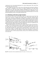
At each node i of the tree, a hyperplane is found that correctly classifies all sam-
ples in one class (this class will be called the “hard"’ class, denoted hc
i
). Then, all
correctly classified samples of the other class (the “soft" class) are removed from

the problem, Fig. (2). The decision of which class is to be assigned “hard" is taken
0 20 40 60 80 100 120 140 160 180 200
0
20
40
60
80
100
120
140
160
180
200
0 20 40 60 80 100 120 140 160 180 200
0
20
40
60
80
100
120
140
160
180
200
Fig. 2. Problem fourclass (Schoelkopf and Smola 2002). Left: hyperplane for the first node.
Right: Problem after first node (“hard" class = triangles).
in a greedy manner for every node (Zapien et al. 2007). The algorithm terminates
when the remaining samples all belong to the same class. Fig.(3) shows a training
sequence. We will further extend this algorithm, but first we give a formalization for

the basic approach.
Problem Statement. Given a two class problem with m = m
1
+ m
−1
samples x
i
∈ R
n
with labels y
i
, i ∈ CC and CC = {1, ,m}. Without loss of generality we define a
Class 1 (Positive Class) CC
1
= {1, ,m
1
}, y
i
= 1 for all i ∈CC
1
, with a global pe-
nalization value D
1
and individual penalization values C
i
= D
1
for all i ∈CC
1
as well

as an analog Class -1 (Negative Class) CC
−1
= {m
1
+ 1, ,m
1
+ m
−1
}, y
i
= −1 for
all i ∈CC
−1
, with a global penalization value D
−1
and individual penalization values
C
i
= D
−1
for all i ∈ CC
−1
.
2.1 Zero vector as solution
In order to train a SVM using the previous definitions, taking one class to be “hard"
in a training step, e.g. CC
−1
is the “hard" class, one could simply set D
−1
→ f and

D
1
<< D
−1
in the primal SVM optimization problem:
minimize
w∈H ,b∈R ,[∈R
m
W(w,[)=
1
2
w
2
+

m
i=1
C
i
[
i
, (3)
subject to y
i
(x
i
,w+ b) ≥1−[
i
, i = 1, ,m, (4)
[

i
≥ 0, i = 1, ,m. (5)
Unfortunately, in some cases the optimization process converges to a trivial solu-
tion: the zero vector. We used the convex hull interpretation of SVMs (Bennett and
14 Janis Fehr, Karina Zapién Arreola and Hans Burkhardt
Fig. 3. Sequence (left to right) of hyperplanes for nodes 1-6 of the tree.
Bredensteiner 2000), in order to determine under which circumstances the trivial so-
lution is occurring and proved the following theorems (Zapien et al. 2007):
Theorem 1: If the convex hull of the “hard" class CC
1
intersects the convex hull of
the “soft" class CC
−1
,thenw = 0 is a feasible point for the primal Problem (4) if
D
−1
≥ max
i∈CC
1
{O
i
}·D
1
, where O
i
are such that
p =

i∈CC
1

O
i
x
i
,
is a convex combination for a point p that belongs to both convex hulls.
Theorem 2: If the center of gravity s
−1
of class CC
−1
is inside the convex hull of
class CC
1
, then it can be written as
s
−1
=

i∈CC
1
O
i
x
i
and s
−1
=

j∈CC
−1

1
m
−1
x
j
with O
i
≥ 0 for all i ∈ CC
1
and

i∈CC
1
O
i
= 1. If additionally, D
1
≥ O
max
D
−1
m
−1
,
where O
max
= max
i∈CC
1
{O

i
},thenw = 0 is a feasible point for the primal Problem.
Please refer to (Zapien et al. 2007) for detailed proofs of both theorems.
2.2 H1-SVM problem formulation
To avoid the zero vector, we proposed a modification of the original SVM optimiza-
tion problem, which is taking advantage of the previous theorems: the H1-SVM (H1
for one hard class).
Fast Support Vector Machine Classification of Very Large Datasets 15
H1-SVM Primal Problem
min
w∈R
n
,b∈R
1
2
w
2
−

i∈CC
¯
k
y
i
(x
i
,w+ b) (6)
subject to y
i
(x

i
,w+ b) ≥1 for all i ∈CC
k
, (7)
where k = 1and
¯
k = −1, or k = −1 and
¯
k = 1.
This new formulation constraints Eq. (7) to classify all samples in the class CC
k
per-
fectly, forcing a “hard" convex hull (H1) for CC
k
. The number of misclassification
on the other class CC
¯
k
is added to the objective function, hence the solution is a
trade-off between a maximal margin and a minimum number of misclassifications in
the “soft" class CC
¯
k
.
H1-SVM Dual Formulation
max
D∈R
m

m

i=1
D
i
−
1
2

m
i, j=1
D
i
D
j
y
i
y
j
x
i
,x
j
 (8)
subject to 0 ≤ D
i
≤C
i
, i ∈CC
k
, (9)
D

j
= 1, j ∈CC
¯
k
, (10)

m
i=1
D
i
y
i
= 0, (11)
where k = 1and
¯
k = −1, or k = −1and
¯
k = 1.
This problem can be solved in a similar way as the original SVM Problem using the
SMO algorithm (Schoelkopf and Smola 2002)(Zapien et al. 2007), and adding some
modifications to force D
i
= 1 ∀i ∈CC
¯
k
.
Theorem 3: For the H1-SVM the zero solution can only occur if |CC
k
|≥(n−1) and
there exists a linear combination of the sample vectors in the “hard" class x

i
∈ CC
k
and the sum of the sample vectors in the “soft" class,

i∈CC
¯
k
x
i
.
Proof: Without loss of generality, let the “hard" class be class CC
1
. Then,
w =
m

i=1
D
i
y
i
x
i
=

i∈CC
1
D
i

x
i
−

i∈CC
−1
D
i
x
i
=

i∈CC
1
D
i
x
i
−

i∈CC
−1
x
i
. (12)
If we define z
i
=

i∈CC

−1
x
i
and |CC
1
|≥(n−1)=dim(z
i
) −1, there exist {D
i
},i ∈
CC
1
,D
i
≡ 0 such that
w =

i∈CC
1
D
i
x
i
−z
i
= 0.
The usual threshold calculation ((Keerthi et al. 1999) and (Schoelkopf and Smola
2002)) can no longer be used to define the hyperplane, please refer to (Zapien et al.
2007) for details on the threshold computation.
The basic algorithm can be improved with some heuristics for greedy ”hard"-class

determination and tree pruning, shown in (Zapien et al. 2007).
16 Janis Fehr, Karina Zapién Arreola and Hans Burkhardt
3 Non-linear extension
In order to classify a sample, one simply runs it down the SVM-tree. When using
only linear nodes, we already obtained good results (Zapien et al. 2006), but we also
observed that first of all, most errors occur in the last node, and second, that over all
only a few samples will reach the last node during the classification procedure. This
motivated us to add a non-linear node (e.g. using RBF kernels) to the end of the tree.
Training of this extended SVM-tree is analogous to the original case. First a pure
SVM
SVM
SVM
label
label
label
label x = −hc
1
label x = −hc
2
label x =

x
i
a SV
D
i
y
i
k(x
i

,x)+b
M
linear SVM: (w
2
,x+b
2
) ×hc
2
> 0
linear SVM: (w
2
,x+b
2
) ×hc
2
> 0
non-linear SVM
Fig. 4. SVM tree with non-linear extesion
linear tree is build. Then we use a heuristic (trade-off between average classification
depth and accuracy) to move the final, non-linear node from the last node up the tree.
It is very important to notice, that to avoid overfitting, the final non-linear SVM has
to be trained on the entire initial training set, and not only on the samples remain-
ing after the last linear node. Otherwise the final node is very likely to suffer from
strong overfitting. Of cause, then the final model will have many SVs, but since only
a few samples will reach the final node, our experiments indicate that the average
classification depth will be hardly affected.
4 Experiments
In order to show the validity and classification accuracy of our algorithm we per-
formed a series of experiments on standard benchmark data sets. These experiments
were conducted

1
e.g. on Faces (Carbonetto) (9172 training samples, 4262 test sam-
ples, 576 features) and USPS (Hull 1994) (18063 training samples, 7291 test sam-
ples, 256 features) as well as on several other data sets. More and detailed exper-
iments can be found in (Zapien et al. 2007). The data was split into training and
test sets and normalized to minimum and maximum feature values (Min-Max) or
standard deviation (Std-Dev).
1
These experiments were run on a computer with a P4, 2.8 GHz and 1G in Ram.
Fast Support Vector Machine Classification of Very Large Datasets 17
Faces RBF H1-SVM H1-SVM RBF/H1 RBF/H1
(Min-Max) Kernel Gr-Heu Gr-Heu
Nr. SVs or 2206 4 4 551.5 551.5
Hyperplanes
Training Time 14:55.23 10:55.70 14:21.99 1.37 1.04
Classification Time 03:13.60 00:14.73 00:14.63 13.14 13.23
Classif. Accuracy % 95.78 % 91.01 % 91.01 % 1.05 1.05
USPS RBF H1-SVM H1-SVM RBF/H1 RBF/H1
(Min-Max) Kernel Gr-Heu Gr-Heu
Nr. SVs or 3597 49 49 73.41 73.41
Hyperplanes
Training Time 00:44.74 00:22.70 02:09.58 1.97 0.35
Classification Time 01:58.59 00:19.99 00:20.07 5.93 5.91
Classif. Accuracy % 95.82 % 93.76 % 93.76 % 1.02 1.02
Comparisons to related work are difficult, since most publications (Bennett and Bre-
densteiner 2000), (Lee and Mangasarian 2001) used datasets with less than 1000
samples, where the training and testing time are negligible. In order to test the per-
formance and speedup on very large datasets, we used our own Cell Nuclei Database
(Zapien et al. 2007) with 3372 training samples, 32 features each, and about 16 mil-
lion test samples:

RBF-Kernel linear tree non-linear tree
H1-SVM H1-SVM
training time ≈1s ≈3s ≈5s
Nr. SVs or 980 86 86
Hyperplanes
average classification - 7.3 8.6
depth
classifiaction time ≈1.5h ≈2 min ≈2 min
accuracy 97.69% 95.43% 97.5%
5 Conclusion
We have presented a new method for fast SVM classification. Compared to non-
linear SVM and speedup methods our experiments showed a very competitive
speedup while achieving reasonable classification results (loosing only marginal
when we apply the non-linear extension compared to non-linear methods). Espe-
cially if our initial assumption holds , that large problems can be split in mainly easy
and only a few hard problems, our algorithm achieves very good results. The ad-
vantage of this approach clearly lies in its simplicity since no parameter has to be
tuned.
18 Janis Fehr, Karina Zapién Arreola and Hans Burkhardt
References
V. VAPNIK (1995): The Nature of Statistical Learning Theory, New York: Springer Verlag.
Y. LEE and O. MANGASARIAN (2001): RSVM: Reduced Support Vector Machines, Pro-
ceedings of the first SIAM International Conference onData Mining, 2001 SIAM Inter-
national Conference, Chicago, Philadelphia.
H. LEI and V. GOVINDARAJU (2005): Speeding Up Multi-class SVM Evaluation by PCA
andFeature Selection, Proceedings of the Workshop on Feature Selection for DataMin-
ing: Interfacing Machine Learning and Statistics, 2005 SIAM Workshop.
C. BURGES and B. SCHOELKOPF (1997): Improving Speed and Accuracy of Support
Vector Learning Machines, Advances in Neural Information Processing Systems9, MIT
Press, MA, pp 375-381.

K. P. BENNETT and E. J. BREDENSTEINER (2000): Duality and Geometry in SVM Clas-
sifiers, Proc. 17th International Conf. on Machine Learning, pp 57-64.
C. HSU and C. LIN (2001): A Comparison of Methods for Multi-Class Support Vector Ma-
chines, Technical report, Department of Computer Science and Information Engineering,
National Taiwan University, Taipei, Taiwan.
T. K. HO AND E. M. KLEINBERG (1996): Building projectable classifiers of arbitrary com-
plexity, Proceedings of the 13th International Conference onPattern Recognition, pp 880-
885, Vienna, Austria.
B. SCHOELKOPF and A. SMOLA (2002): Learning with Kernels, The MIT Press, Cam-
bridge,MA, USA.
S. KEERTHI and S. SHEVADE and C. Bhattacharyya and K. Murthy (1999): Improvements
to Platt’s SMO Algorithm for SVM Classifier Design, Technical report, Dept. ofCSA,
Banglore, India.
P. CARBONETTO: Face data base, pcarbo/, University of British
Columbia Computer Science Deptartment.
J. J. HULL (1994): A database for handwritten text recognition research, IEEE Transactions
on Pattern Analysis and Machine Intelligence, Vol 16, No 5, pp 550-554.
K. ZAPIEN, J. FEHR and H. BURKHARDT (2006): Fast Support Vector Machine Classifi-
cation using linear SVMs, in Proceedings: ICPR, pp. 366- 369 ,Hong Kong 2006.
O. RONNEBERGER and et al.: SVM template library, University of Freiburg, Depart-
ment of Computer Science, Chair of Pattern Recognition and Image Processing,
/>K. ZAPIEN, J. FEHR and H. BURKHARDT (2007): Fast Support Vector Machine Classi-
fication of very large Datasets, Technical Report 2/2007, University of Freiburg, De-
partment of Computer Science, Chair of Pattern Recognition and Image Processing.
/>Fusion of Multiple Statistical Classifiers
Eugeniusz Gatnar
Institute of Statistics, Katowice University of Economics,
Bogucicka 14, 40-226 Katowice, Poland

Abstract. In the last decade the classifier ensembles have enjoyed a growing attention and

popularity due to their properties and successful applications.
A number of combination techniques, including majority vote, average vote, behavior-
knowledge space, etc. are used to amplify correct decisions of the ensemble members. But the
key of the success of classifier fusion is diversity of the combined classifiers.
In this paper we compare the most commonly used combination rules and discuss their
relationship with diversity of individual classifiers.
1 Introduction
Fusion of multiple classifiers is one of the recent major advances in statistics and ma-
chine learning. In this framework, multiple models are built on the basis of training
set and combined into an ensemble or a committee of classifiers. Then the component
models determine the predicted class.
Classifier ensembles proved to be high performance classification systems in nu-
merous applications, e.g. pattern recognition, document analysis, personal identifi-
cation, data mining etc.
The high accuracy of the ensemble is achieved if its members are “weak" and di-
verse. The term “weak” refers to unstable classifiers, such as classification trees, and
neural nets. Diversity means that the classifiers are different from each other (inde-
pendent, uncorrelated). This is usually obtained by using different training subsets,
assigning different weights to instances or selecting different subsets of features.
Tumer and Ghosh (1996) have shown that the ensemble error decreases with the
reduction in correlation between component classifiers. Therefore, we need to assess
the level of indpendence of the members of the ensemble, and different measures of
diversity have been proposed so far.
The paper is organised as follows. In Section 2 we give some basics on classi-
fier fusion. Section 3 contains a short description of selected diversity measures. In
Section 4 we discuss the fusion methods (combination rules). The problems related
20 Eugeniusz Gatnar
to assessment of performance of combination rules and their relationship with diver-
sity measures are presented in Section 5. Section 6 gives a brief description of our
experiments and the obtained results. The last section contains some conclusions.

2 Classifier fusion
A classifier C is any mapping C : X →Y from the feature space X into a set of class
labels Y = {l
1
,l
2
, ,l
J
}.
The classifier fusion consists of two steps. In the first step the set of M in-
dividual classifiers {C
1
,C
2
, ,C
M
} is designed on the basis of the training set
T = {(x
1
,y
1
),(x
2
,y
2
), ,(x
N
,y
N
)}.

Then, in the second step, their predictions are combined into an ensemble
ˆ
C
∗
using a combination function F:
ˆ
C
∗
= F(
ˆ
C
1
,
ˆ
C
2
, ,
ˆ
C
M
). (1)
Various combinatorial rules have been proposed in the literature to approximate the
function F, and some of them will be discussed in Section 4.
3 Diversity of ensemble members
In order to assess the mutual independence of individual classifiers, different mea-
sures have been proposed. The simplest ones are pairwise measures defined between
two classifiers, and the overall diversity of the ensemble is the average of the diver-
sities (U) between all pairs of the ensemble members:
Diversity(C
∗

)=
2
M(M −1)
M−1

m=1
M

k=m+1
U(m,k). (2)
The relationship between a pair of classifiers C
i
and C
j
can be shown in the form
of the 2 ×2 contingency table (Table 1).
Table 1. A2×2 contingency table for the two classifier outputs.
Classifiers C
j
is correct C
j
is wrong
C
i
is correct a b
C
i
is wrong c d
The well known measure of classifier dependence is the binary version of the
Pearson’s correlation coefficient:

r(i, j)=
ad −bc

(a + b)(c + d)(a+c)(b+d)
. (3)
Fusion of Multiple Statistical Classifiers 21
Partridge and Yates (1996) have used a measure named within-set generalization
diversity. This measure is simply the kappa statistics:
N(i, j)=
2(ac −bd)
(a + b)(c + d)+(a+c)(b+d)
. (4)
Skalak (1996) reported the use of the disagreement measure:
DM(i, j)=
b + c
a + b + c + d
. (5)
Giacinto and Roli (2000) have introduced a measure based on the compound
error probability for the two classifiers, and named compound diversity:
CD(i, j)=
d
a + b + c + d
. (6)
This measure is also named “double-fault measure” because it is the proportion of
the examples that have been misclassified by both classifiers.
Kuncheva et al. (2000) strongly recommended the Yule’s Q statistics to evaluate
the diversity:
Q(i, j)=
ad −bc
ad + bc

. (7)
Unfortunately, this measure has two disadvantages. In some cases its value may be
undefined. e.g. when a = 0andb = 0, and it cannot distinguish between different
distributions of classifier outputs.
In order to overcome the drawbacks of the Yule’s Q statistics, Gatnar (2005)
proposed the diversity measure based on the Hamann’s coefficient:
H(i, j)=
(a + d)−(b+ c)
a + b + c + d
. (8)
Several non-pairwise measures have been also developed to evaluate the level of
diversity between all members of the ensemble.
Cunningham and Carney (2000) suggested using the entropy function:
EC = −
1
N
N

i=1
L(x
i
)log(L(x
i
)) −
1
N
N

i=1
(M −L(x

i
))log(M −L(x
i
)), (9)
where L(x) is the number of classifiers that correctly classified the observation x.Its
simplified version was introduced by Kuncheva and Whitaker (2003):
E =
1
N
N

i=1
1
M −M/2
min{L(x
i
),M −L(x
i
)}. (10)
Kohavi and Wolpert (1996) used their variance to evaluate the diversity: