GIS Methodologies for Developing Conservation Strategies Part 7 doc
Bạn đang xem bản rút gọn của tài liệu. Xem và tải ngay bản đầy đủ của tài liệu tại đây (392.18 KB, 27 trang )
140 Lambert and Carr
hoped that analysis and mapping of a corridor network would assist Central
American governments and nongovernmental organizations in the identification
and prioritization of key areas for preservation and protection. A spin-off benefit
of this project is a preliminary GIS database of the entire Central American
isthmus which has been shared with many government agencies in Central
America, other scientists, land use planners, and conservation organizations
that are also working to preserve and manage the natural treasures of Central
America.
Database Development and Evaluation
The GIS database development component of the corridor study was designed
as a two-phase process to complement the preliminary and more detailed analy-
sis efforts. Initially, due to limited funding, only the data layers that were re-
quired to support the preliminary corridor potential study would be developed.
Subsequently, with additional funding, the team would develop more compre-
hensive databases to support more detailed study of specific potential linkages.
The logical first step for the team was the identification and collection of
existing digital data sources that could be obtained inexpensively. Unfortunately,
the team found that, although there were several GIS projects being conducted
in Central America, the GIS databases these projects were creating varied widely
in scale, projection, content, theme, date, and digital format. There were appar-
ently no regional efforts being made to develop a standardized database for the
entire isthmus.
Fortunately, an affordable source for base map features called the Digital
Chart of the World (DCW) had just become available (ESRI 1993). The DCW
provides base map features such as roads, hydrography, political boundaries,
population centers, and topography (at 1,000-foot intervals) for the entire world.
This database was created by digitizing the U.S. Defense Mapping Agency’s
1:1,000,000 scale Operational Navigation Chart map series. A license for the
ARC/INFO version of the DCW database was purchased from Environmental
Systems Research Institute, Inc. (ESRI) in the fall of 1992. At first, the team was
skeptical about the suitability of this database because the scale of the source
data limits typical spatial accuracy to approximately plus/minus one kilometer.
However, the alternative of digitizing base map features for all of Central
America motivated the team to test the database. After working with the data-
base, the team found the DCW’s spatial and attribute accuracy to be quite
adequate and appropriate for the objectives of this preliminary, multinational
study.
An important point to make about the DCW is that its availability allowed
The Paseo Pantera Project 141
the planning team to concentrate its own limited funding on the generation of
the new databases required for analysis and on the preliminary design of the
corridor rather than on the digitizing of base map feature layers. However, a
second important advantage to using the DCW was that it allowed the team to
get off to a quick start. All too often in the past, ambitious GIS managers have
promoted this technology successfully to their cautious colleagues, only to find
themselves explaining later, to now impatient colleagues, why it takes so long to
demonstrate any substantial results from a technology that was supposed to save
time and increase productivity. Being aware of this potential scenario, and the
fact that GIS technology and methods are still new to many of the participants in
the Paseo Pantera project (especially some of the cooperating institutions in
Central America), the corridor planning team recognized the need to demon-
strate the utility of GIS as quickly as possible to its sponsors. The DCW made this
possible. Although the DCW will not be appropriate for all projects, this project
demonstrates the potential value of the DCW to those faced with continental-
scale environmental problems and dwindling budgets.
The second step in the initial phase of GIS database development involved
the team in a process of weighing the costs of producing each new data layer
against the relative potential contribution of that data to the preliminary analysis.
Several new data layers were subsequently developed, including boundaries
of existing and proposed protected areas; forested/deforested areas; potential
biological communities based on the Holdridge system of life zone classifications
(Holdridge 1967); population density and major population centers; and areas
occupied by indigenous populations. The GIS data layers listed above represent
the conversion of more than seventy-five source maps to digital format. It is
important to point out that these data sets represent only a preliminary effort,
limited by modest funding, and that the study team recognizes the need for
much more detailed information as it enters the second phase of this study.
Once the databases described above were developed, the team explored ways
to use them to analyze the potential for a continuous biological corridor. The
following four criteria were selected for use in the model based on the evaluation
of the available data: (1) size of protected areas, (2) uniform national designation
of protected areas, (3) population densities, and (4) forested/deforested areas.
The protected areas were divided into two size classes—large (50,000 hectares
and greater) and small (less than 50,000 hectares). These classes were based on
suggestions for minimum core area size in Noss (1991).
Because of the variations in terminology used by each country to classify its
protected areas, the team developed a set of “uniform national designations”
based on current management practices. These designations were: national park
(or equivalent), anthropological reserve, extractive reserve, private reserve, and
proposed reserve. “Uniform national designation” was selected as an important
criterion because the management practices used in each protected area deter-
142 Lambert and Carr
mine its value to the preservation of biological diversity. An uninhabited national
park will contribute differently than an inhabited anthropological reserve.
Owing to variations in the ranges used for population density categories
for each country, the team had to determine a generalized population density
classification scheme for the entire region. Five density classes were used, with
the following ranges: 0 to 10 people per square kilometer, 11 to 25, 26 to 50, 51 to
100, and 101 people or more per square kilometer. Population density was
considered a critical criterion because, according to Redford and Robinson (1992),
where densities are higher there is less potential to maintain biodiversity.
The fourth criterion utilized in the preliminary analysis was the classification
of “forested/deforested” (or natural/altered) areas. This generalized data was
digitized from the map supplement (“The Coexistence of Indigenous Peoples
and the Natural Environment in Central America”) contained in the spring 1992
issue of Research and Exploration, a publication of the National Geographic Society.
This classification was considered to be a significant discriminator, at this resolu-
tion of analysis, because it is generally accepted that natural areas will have
higher “natural diversity” than deforested, human-altered areas.
After an evaluation of the remaining available spatial databases, several were
not used in the model developed for our initial analyses because of their incom-
plete classification or content. These data sets included roads, hydrography, and
population centers. Holdridge’s life zones and areas of indigenous populations
were not used because the team could not substantiate the prioritization of one
life zone over another, and there was controversy over whether or not historical
ranges of indigenous populations were predictive of corridor potential.
Biological Corridor Suitability, Potential, and Feasibility Analyses
All analysis from this point in the method was accomplished by using ESRI’s
raster GIS software called GRID. The vector data layers used in the analysis were
converted into layers of four-square-kilometer grid cells. This was the highest
reasonable resolution based on the spatial accuracy of the combined source data
layers.
A weighted criteria analysis method was used to generate a biological corri-
dor suitability map that would subsequently be used as an input to the corridor
potential and feasibility analyses. There were three steps in the weighted criteria
analysis. The first was to determine the relative values for the range of options
within each of the four criteria discussed above. The second was to determine
the relative importance among the four criteria (i.e., to assign a weight to each
criteria). The third was to calculate the normalized, cumulative scores, which
results in values ranging from 1 to 100. These values represent the relative overall
The Paseo Pantera Project 143
suitability of any area for inclusion in a biological corridor. Several alternative
weighting schemes have been explored for assigning the values within and
among the criteria.
In the first step, for the criterion of “size of protected area,” lands contained
in larger protected areas were considered relatively more valuable than lands
found in smaller protected areas, based on theories put forth by MacArthur and
Wilson (1967). Lands with no protection received the lowest relative value for
this criterion. Similarly, for the criterion of “uniform national designation,” lands
in “national park (or equivalent)” were determined to be of highest value, lands
in “proposed reserves” to be of a lower value, and lands not in a protected area
to be of no relative value. For each category of protected area, the stricter the
limits on use (as determined by management practices), the more important its
potential contribution to protection of biodiversity was considered to be. Within
the criterion for population density, areas of high density were considered to be
a detriment to the development of a corridor network, whereas low-density areas
were assumed to be of higher relative value. Finally, lands with natural forest
cover were considered to be of much greater relative value than altered lands.
The corridor suitability database provided the relative cost information
needed for the next step in the corridor analysis. The cells with high corridor
suitability were redefined as cells with low relative “costs” for inclusion in the
corridor. The cells with low corridor suitability were redefined as having high
relative “costs” for inclusion. The resulting “cost” surface was the input for the
assessment of corridor potential. This analysis used the GRID analysis function
corridor to calculate the relative accumulated “cost” of developing a corridor
between two sources. In this case, the two sources were Mexico and Colombia.
The corridor function generated a value for each four-square-kilometer pixel
along the least cost path to each of the sources. In figure 11.1, the values have
been divided into five classes of equal area. These results represent continuous
biological corridor potential based on the criteria used.
The areas of highest corridor potential were not simply along the shortest
route between Colombia and Mexico, but represented a combination of distance
and other influences assigned through the four criteria used in the weighted
criteria analysis. The result was a bias toward large, forested national parks with
low population density in close proximity.
In the final step of the analysis, the boundaries of the area represented by the
classes of highest corridor potential were used to “clip out” the corresponding
suitability classifications developed in the weighted criteria analysis step. The
resulting map (figure 11.2) represents biological corridor feasibility. The area
within these limits had the highest potential for a continuous corridor, but the
feasibility factor was not homogeneous within the limits. Three problem areas
became evident: one in northwestern Honduras, another in northeastern Costa
Rica, and the third around the Panama Canal.
144 Lambert and Carr
Conclusions from the Initial Corridor Study and Thoughts on the
Next Phase of Study
The authors believe that the methods they used for this preliminary study have
great potential to assist in the identification of corridor study areas and in
their prioritization. The maps and reports generated from these preliminary (but
promising) results have been used widely throughout Central America and the
United States to promote the concept of a Mesoamerican biological corridor.
There has also been greater appreciation of the contribution that GIS technology
can make to conservation planning. The study team is currently focusing on
refinements to its methodology to strengthen the relationships between current
F
IG.
11.1 The continuous biological corridor potential in Central America (based
upon criteria described in the text)
The Paseo Pantera Project 145
scientific theories and the relative weights assignments, and on the development
of new and improved data sets to support more detailed planning.
As a result of its experience with this study, the team has recommended the
use of, and begun development of, 1:250,000 scale data sets to support the next,
more detailed phase of regional corridor analysis. A second-phase pilot project,
implemented at this scale, was completed by the authors in the fall of 1995 for
the trinational region of the Selva Maya (which includes Belize, the Peten district
of Guatemala, and southern Mexico). This project was supported by the MAYA-
FOR program of USAID / G-CAP. The GIS database was created for the planning
of biological corridors but has also been used more generally to support the
Regional Conservation Assessment Workshop for the Maya Tropical Forest held
in San Cristobal de las Casas, Chiapas, Mexico, in August 1995. This workshop
F
IG.
11.2 Corridor feasibility analysis results
146 Lambert and Carr
brought together more than sixty representatives from the region to establish
conservation needs and priorities for the Selva Maya. The new standardized
multinational GIS database provided the participants with a common base map
and data which enabled multinational conservation planning that would not
have been possible before. Instead of dealing with a different map for each
country, the regional database allowed the participants to more effectively plan
strategies based on ecological boundaries rather than political boundaries. Addi-
tionally, the new standardized database was distributed to over thirty govern-
mental, academic, and conservation institutions in the region in the hopes that
their future conservation planning efforts would not be limited by national
boundaries.
Based on the experience gained through implementing the MAYAFOR GIS
database, the authors recommend that a coordinated and cooperative effort be
initiated whereby a standardized GIS database would be developed for the entire
isthmus. It is further recommended that this database be freely shared with any
parties involved in conservation of the region’s natural resources in order to
prevent duplication of effort and to make efficient use of limited funding. The
team believes that a 1:250,000 scale database has been shown to provide sufficient
detail and accuracy for many regional conservation planning needs and is rea-
sonable to develop within the limited funding constraints of the conservation
community.
References
Carr III, A. F. 1992. Paseo Pantera Project brochure. New York: Wildlife Conservation
Society.
Carr, M. H., J. D. Lambert, and P. D. Zwick. 1994. Mapping of biological corridor potential
in Central America. In A. Vega, ed., Conservation corridors in the Central American
region, 383–93. Gainesville, Fla.: Tropical Research and Development.
Environmental Systems Research Institute (ESRI). 1993. Digital chart of the world (CD-ROM
Cartographic Database). Redlands, Calif.: ESRI.
Forman, R. T. T. and M. Godron. 1986. Landscape ecology. New York: Wiley.
Harris, L. D. and K. Atkins. 1991. Faunal movement corridors in Florida. In W. E. Hudson,
ed., Landscape linkages and biodiversity, 117–38. Washington, D.C.: Island Press.
Holdridge, L. R. 1967. Life zone ecology. San Jose
´
, C.R.: Tropical Science Center.
Lambert, J. D. and M. Carr. 1993 (May). Utilizing GIS to plan for a Central American
biological corridor. Proceedings, Thirteenth Annual ESRI User Conference 1: 257–64. Red-
lands, Calif.: Environmental Systems Research Institute.
MacArthur, R. H. and E. O. Wilson. 1967. The theory of island biogeography. Princeton:
Princeton University Press.
Noss, R. F. 1991. Landscape connectivity: Different functions at different scales. In W. E.
Hudson, ed., Landscape linkages and biodiversity, 27–39. Washington, D. C.: Island Press.
The Paseo Pantera Project 147
Redford, K. H. and J. G. Robinson. 1992. The sustainability of wildlife and natural areas.
Proceedings of the International Conference on the Definition and Measurement of Sus-
tainability, Washington, D.C.
Soule
´
, M. E. 1991. Theory and strategy. In W. E. Hudson, ed., Landscape linkages and
biodiversity, 91–104. Washington, D.C.: Island Press.
This page intentionally left blank
Part Four
The USAID Case Study in
Gap Analysis
This page intentionally left blank
12
Overview of Gap Analysis
Basil G. Savitsky
Gap analysis is a “search for biotic communities and species in need of preserva-
tion management” (Davis et al. 1990:56). Gap analysis provides a method for
assessing present measures to protect biological diversity and for identifying
focus areas for optimal conservation efforts (Scott et al. 1987). Gap analysis is a
GIS technique which superimposes species distributions with boundaries of
ecosystems and protected areas to identify gaps in the protection of species. GIS
is used to overlay maps or layers that are geographically referenced to each other
and to create new information through the combination of those map files. Image
analysis is used to create the vegetation database that provides the framework
for the various GIS data layers. GPS has been used in conjunction with field
components of image analysis and is beginning to be utilized as a wildlife data
collection technology.
One tool that was developed during this project was the Habitat Conserva-
tion Decision Cube. The decision cube is covered in detail in chapter 15, but is
introduced at this time as it defined the database design for the USAID project.
The decision cube can be represented as a three-dimensional box with eight
internal cubes (see figure 15.2). The eight cubes represent possible outcomes
when three separate axes are viewed for the presence or absence of the three
variables used in gap analysis. The three variables are the presence or absence of
a species or group of species of wildlife; the presence or absence of suitable
habitat for that species; and the presence or absence of protected areas. Each of
the eight types of locations require different policy approaches. For example, gap
analysis was designed to identify the locations where species and habitat are
present that are outside of protected areas. Such locations adjacent to or between
protected areas are prioritized in land acquisitions for conservation purposes.
152 Basil G. Savitsky
History and Status
There is growing recognition in the United States of the high cost and low
efficiency of the species level approach to conservation of biological diversity
associated with the 1973 Endangered Species Act (Edwards et al. 1995). Gap
analysis is one approach in extending conservation of biological diversity from
reactive legislative battles over individual species to strategic planning for habitat
conservation.
The methodology for gap analysis is based upon the logic used in evaluating
the representation of vegetation communities within protected areas, such as
studies performed in the United States (Crumpacker et al. 1988) and Africa
(Huntley 1988). Evaluation of wildlife in a gap analysis framework was first
performed in the United States in a study in Hawaii. The measurement of the
geographic intersection of the home range of endangered forest bird species with
protected areas indicated that less than 10 percent of the bird habitat was pro-
tected (Scott et al. 1987). In 1989 Idaho initiated a statewide gap analysis project
which addressed a wide variety of wildlife species and habitat. Since that time,
gap analysis projects have been completed for most of the western states in the
United States.
Gap analysis is a technique that is receiving a high level of attention from
conservation agencies and organizations (Machlis, Forester, and McKendry 1994).
It is an effective tool for decision-makers and policy analysts because it clearly
maps out potential conservation priorities and the path used to reach those
priorities. Gap analysis results can be combined with economic development
needs as constraints or opportunities in geographic selection of sustainable devel-
opment projects. Thus, gap analysis is likely to be a focal technique in biodiver-
sity and sustainable development research in the future.
The Application of Gap Analysis in the United States
Gap analysis is a biodiversity planning approach which has been embraced by
the U. S. Geological Survey, Biological Resources Division (Machlis, Forester, and
McKendry 1994). The state of Utah published a report that contained four maps,
two CD-ROMs, and documentation of the methodology used and results ob-
tained (Edwards et al. 1995). The four maps include a mosaic of Landsat TM
images, habitat classes generated from the image analysis, distribution of public
lands, and a combination of habitat data and public lands suitable for consider-
ation in wildlife management plans. The two CD-ROMs contain data on the
distribution of 525 wildlife species.
A gap analysis also has been completed for the southwestern portion of
Overview of Gap Analysis 153
the state of California (Davis 1994). The project identified eighteen vegetation
communities and forty-two vertebrate species at risk in the region. The minimum
mapping unit for the project was one square kilometer (100 hectares), and final
results were presented at a scale which utilized 7.5 minute U.S. Geological Survey
topographic quadrangle maps as the smallest geographic unit of analysis.
The state of Florida performed a gap analysis for 120 vertebrate species (Cox
et al. 1994). This gap analysis was only a subset of the extensive wildlife and
habitat analyses performed by the state. Biological data holdings in Florida are
rich, with over 25,000 geographically referenced locations of rare plants, animals,
and natural communities. These data were combined with statewide land cover
maps generated from Landsat imagery to identify strategic habitat conservation
areas and a separate set of maps indicating regional diversity hot spots.
International Application of Gap Analysis
Gap analysis projects are beginning to be performed in tropical developing
countries. Two Latin American projects have used GIS to present existing biodi-
versity data and to integrate these data for preliminary strategic assessments.
One example of this level of mapping is “Biological Priorities for Conservation
in Amazonia” (Conservation International 1991). The content of this map was
based upon a workshop of zoologists, systemic botanists, and vegetation ecolo-
gists. The geographic methodology utilized in the integration of biological and
protected area data was innovative, and the project is sure to be followed with
more detailed assessments. However, it should be noted that a map at a scale of
1:5,000,000 is useful only in very broad identification of conservation priorities.
The general scale of this level of analysis is evidenced by the fact that the entire
country of Costa Rica is smaller than several of the high-priority conservation
regions identified in Amazonia.
A more detailed project was performed in Costa Rica (Fundacio
´
n Neotro
´
pica
and Conservation International 1988). Priority conservation regions were identi-
fied by superimposing data on the percentage of natural vegetation cover with
boundaries of watersheds and protected areas. Although the scale of the vegeta-
tion maps used in the study was 1:200,000, the only wildlife data utilized were
locations of endangered, threatened, and rare species. The objective of the study
was to compare thirty-three watershed units in order to identify national priori-
ties in watershed management.
Both the Amazonia and Costa Rica projects were able to provide only general
information on biological diversity because they were limited in available details
on either habitat or wildlife data. This author has observed that biodiversity
projects in the tropics either have not utilized all of the data layers used in gap
analysis projects in the United States (wildlife, habitat, and protected areas) or
154 Basil G. Savitsky
they have not yet been able to utilize a scale of analysis as detailed as projects in
the United States. This project in Costa Rica utilized the habitat and protected
area data at a similar scale of analysis as other gap analysis projects in the United
States. Since a national survey of wildlife was performed, the wildlife data in the
Costa Rica project had a greater level of depth than U.S. gap analysis projects.
However, because only twenty-one species of wildlife were evaluated, the level
of breadth was lower than most gap analysis projects in the United States. The
extent to which the international application of detailed gap analysis becomes
more frequent may depend in large part on the ability of the international
community to produce viable habitat maps for use in national conservation
efforts.
There are positive indications that the international community is moving
toward funding projects that will generate regional databases useful for detailed
biodiversity assessments such as national gap analyses. Several regional habitat
mapping projects (detailed in chapter 5) are being proposed or are in early
phases. The 1992 United Nations Conference on Environment and Development
(UNCED) drafted Agenda 21, a list of action areas for creating a sustainable
future. Agenda 21 addresses biodiversity and information for decision making as
two of its twenty-eight platform areas (Parson, Haas, and Levy 1992). The fact
that biodiversity is one of four categories funded through the Global Environ-
ment Facility (Reed 1991) is indicative of the strategic direction and intention of
the United Nations Environment Program, the United Nations Development
Program, and the World Bank. All of these mechanisms indicate that natural
resource managers in developing tropical countries may have more and better
habitat data in the near future upon which to build national analyses. It remains
the responsibility of the national agencies, private conservation groups, and
academic institutions to collect or integrate the wildlife data.
Critique of Gap Analysis
Gap analysis has been shown to be an effective tool for conservation assessment
in statewide applications within the United States. GIS has served as a useful
mechanism both for integrating data on wildlife, habitat, and protected areas and
for providing mapped information for strategic conservation planning. There is
interest in combining the gap analysis model with socioeconomic models to
better understand our choices in human-environmental interactions (McKendry
and Machlis 1991; Machlis, Forester, and McKendry 1994). This level of interdisci-
plinary research is indicative of the utility of the gap analysis model in providing
biodiversity information that is useful in a broad decision-making context.
Nevertheless, there are numerous limitations to the use of the gap analysis
Overview of Gap Analysis 155
model (Scott et al. 1993), and these are discussed in detail in chapter 14. However,
three constraints to the application of the model are noted here. First, since gap
analysis is a coarse planning tool designed to indicate regional patterns, results
need to be interpreted accordingly and verified in the field at a finer scale of
analysis. Second, gap analysis is intended to augment rather than replace efforts
to identify and protect individual species of concern and centers of endemism.
Third, gap analysis provides information on geographic areas possibly worth
adding to the system of protected areas from the biological perspective. Success-
ful implementation of a land acquisition strategy requires data on land owner-
ship which may or may not be readily available for use in a digital format.
Definition of Terms and Concepts
Several terms used throughout the balance of the USAID case study are defined
below:
Biolo gical Diver sity
Biological diversity has been defined along three hierarchical categories as “the
totality of genes, species, and ecosystems in a region” (WRI/IUCN/UNEP
1992:2) The unit of measurement for genetic diversity is either a population or a
species. Species diversity is measured within the region of the ecosystem. The
region for measuring ecosystem diversity is not as well defined as the regions for
the other two units, but it is generally understood to be applied at the national
or subnational level. Gap analysis utilizes species diversity data to depict geo-
graphic pattern at the ecosystem-diversity scale of analysis.
Mappi ng of Habitat, Land Cover, Land Use, and Vegetat ion
Although there are differences between these four terms, they are used synony-
mously in this text. The same feature, such as a patch of forest, can be found in
the classification schemes of each of the four types of maps. For example, the
land cover of forest vegetation, when it occurs within an urban land use (such as
a residential neighborhood or a city park), is classified as urban habitat. The
focus of the project was on mapping the distribution of vertebrate species that
are closely linked to forested habitat. This study does not address variation
within forests, such as undisturbed or secondary growth forests.
Prote cted Areas
There are five protected area management categories which the World Conserva-
tion Union (IUCN) employs. These categories are: strict nature reserves, national
parks, natural monuments, habitat and wildlife management areas, and pro-
156 Basil G. Savitsky
tected landscapes (WRI/IUCN/UNEP 1992). Although the wildlife conservation
objectives of these five categories vary, all protected areas are treated equally in
the context of this gap analysis project.
Regio nal Landsca pe
The question of scale is at the heart of the discipline of geography. One review of
the use of spatial scale in conservation biology concludes that “landscape is the
preferable term for describing large natural areas with conservation value” (Csuti
1991:81). Further,
The regional landscape (generally in the range of 1,000 to 100,000 square
kilometers) is a convenient scale at which to integrate planning and manage-
ment for multiple levels of organization. It is the scale of a constellation of
national forests, parks, and surrounding private lands, or of a large watershed
or mountain range. The regional landscape is big enough to comprise numer-
ous, interacting ecosystems; to incorporate large natural disturbances; and to
maintain viable populations of large, wide-ranging animals. Yet, it is small
enough to be biogeographically distinct, and to be mapped in detail and
managed by people who know the land well. (Noss 1992:241)
Policy relevant to biodiversity should be formulated at the landscape scale in
order to focus on the processes of ecosystem health across human generations
rather than on the protection of individual species (Norton and Ulanowicz 1991).
References
Conservation International. 1991. Biological priorities for conservation in Amazonia. Map
printed at a scale of 1:5,000,000. Washington, D.C.: Conservation International.
Cox, J., R. Kautz, M. MacLaughlin, and T. Gilbert. 1994. Closing the gaps in Florida’s wildlife
habitat conservation systems. Tallahassee, Fla.: Office of Environmental Services.
Crumpacker, D. W., S. W. Hodge, D. Friedley, and W. P. Gregg, Jr. 1988. A preliminary
assessment of the status of major terrestrial and wetland ecosystems on federal and
Indian lands in the United States. Conservation Biology 2: 103–15.
Csuti, B. 1991. Conservation corridors: Countering habitat fragmentation. In W. E. Hud-
son, ed., Landscape linkages and biodiversity, 81–90. Washington, D.C.: Island Press.
Davis, F. W. 1994. Gap analysis of the southwestern California region. Technical Report 94–4.
Santa Barbara, Calif.: National Center for Geographic Information and Analysis.
Davis, F. W., D. M. Stoms, J. E. Estes, J. Scepan, and J. M. Scott. 1990. An information
systems approach to the preservation of biological diversity. International Journal of
Geographical Information Systems 4: 55–78.
Edwards, T. C. Jr., C. G. Homer, S. C. Bassett, A. Falconer, R. D. Ramsey, and D. W. Wight.
1995. Utah gap analysis: An environmental information system. Final Project Report 95–1.
Logan: Utah Cooperative Fish and Wildlife Research Unit.
Fundacio
´
n Neotro
´
pica and Conservation International. 1988. Costa Rica: Assessment of the
Overview of Gap Analysis 157
conservation of biological resources (thirteen pages and four maps at 1:909,091 scale). San
Jose
´
, C.R.: Fundacio
´
n Neotro
´
pica.
Huntley, B. J. 1988. Conserving and monitoring biotic diversity: Some African examples.
In E. O. Wilson, ed., Biodiversity, 248–60. Washington, D.C.: National Academy Press.
Machlis, G. E., D. J. Forester, and J. E. McKendry. 1994. Biodiversity gap analysis: Critical
challenges and solutions. Moscow: University of Idaho.
McKendry, J. E. and G. E. Machlis. 1991. The role of geography in extending biodiversity
gap analysis. Applied Geography 11: 135–52.
Norton, B. G. and R. E. Ulanowicz. 1991. Scale and biodiversity policy: A hierarchical
approach. Ambio 21: 244–49.
Noss, R. F. 1992. Issues of scale in conservation biology. In P. L. Fiedler and S. K. Jain, eds.,
Conservation biology, 239–50. New York: Chapman and Hall.
Parson, E. A., P. M. Haas, and M. A. Levy. 1992. A summary of the major documents
signed at the earth summit and the global forum. Environment 34 (August): 12–36.
Reed, D. 1991. The Global Environment Facility: Sharing responsibility for the biosphere. Wash-
ington, D. C.: World Wildlife Fund—International.
Scott, J. M., B. Csuti, J. D. Jacobi, and J. E. Estes. 1987. Species richness: A geographic
approach to protecting future biological diversity. BioScience 37: 782–88.
Scott, J. M., F. Davis, B. Csuti, R. Noss, B. Butterfield, C. Groves, H. Anderson, S. Caicco,
F. D’Erchia, T. C. Edwards Jr., J. Ulliman, and R. G. Wright. 1993. Gap analysis: A
geographical approach to protection of biological diversity. Wildlife Monograph no. 123 (41
pp.). Bethesda, Md.: The Wildlife Society.
World Resources Institute (WRI), World Conservation Union (IUCN), United Nations
Environment Programme (UNEP). 1992. Global biodiversity strategy: Guidelines for action
to save, study, and use Earth’s biotic wealth sustainably and equitably. Washington, D.C.:
WRI.
13
Wildlife and Habitat Data Collection
and Analysis
Basil G. Savitsky, Jorge Fallas, Christopher Vaughan,
and Thomas E. Lacher Jr.
Development of Habitat and Wildlife Databases
Costa Rica, with an area of only 51,100 km
2
, has one of the highest levels of
biodiversity per unit area in the world. According to the Holdridge system of life
zones (Holdridge 1967), Costa Rica can be divided into twenty-four life zones,
each of which possesses unique characteristics of elevation, temperature, precipi-
tation, and evapotranspiration potential. This high diversity of environmental
conditions has generated an equally diverse landscape with an extremely high
diversity of plants and animals. Not all species could be included in a wildlife
database, and a decision needed to be made concerning the level of detail of the
habitat map that would be used as well. This chapter discusses the relevant
issues for the creation of wildlife and habitat databases.
Habitat Map
One of the research objectives was to create a habitat map of Costa Rica and
superimpose it with map layers on wildlife and protected areas to perform a
national gap analysis of Costa Rica. The purpose of the habitat map is to provide
a polygon-structured base map to which point-structured wildlife data are re-
lated. The polygons need to contain data that are specific enough to be meaning-
ful in diagnosing spatial trends in the wildlife data, but general enough to be
manageable in addressing a national database. A target scale of 1:200,000 was
Data Collection and Analysis 159
selected for the habitat map because the wildlife data and a variety of other data
sources were available at this scale. A flow chart of the procedures used to create
the habitat map is provided (figure 13.1).
The initial compilation of the habitat map was based upon an unpublished
land use and land cover map of Costa Rica produced by the Instituto Geogra
´
fico
Nacional de Costa Rica (IGN 1984). The IGN map series contained data on the
distribution of forty land use and land cover categories at a scale of 1:200,000. In
order to approximate the desired classes in the habitat map, the forty classes
were generalized using color pens to a set of maps containing eleven classes
defined as 1984 Land Use (table 13.1). Boundaries of the simplified polygons
were transferred to mylar transparencies. The line work was digitized, and the
polygons were labeled using ARC/INFO software. The data were then placed in
a grid of 28.5 meter cells and exported to the format of ERDAS software in order
to be used in the image analysis of more recent TM data.
The 1984 land use data were confirmed and updated using Landsat TM data.
A computer search of all available TM imagery was performed to identify the
most cloud-free scenes. Five TM scenes were acquired from 1991–92, providing
coverage of the entire country of Costa Rica. The TM images were geographically
referenced to 1:50,000 scale topographic maps. Thus, habitat classification maps
resulting from TM image interpretation could be generalized to a scale of
1:200,000. Image analysis performed at Clemson University was directed toward
a general classification of the imagery for the entire country. Image analysis
performed at the Universidad Nacional Autonoma de Costa Rica (UNA) was
directed toward providing a more detailed classification of two of the five TM
scenes.
The national classification was performed using an unsupervised classifica-
tion technique. In order to label the unsupervised classes, the land use data were
overlaid with the TM classified data. Output from the unsupervised classification
resulted in a map indicating forest, nonforest, water, and clouds.
The four-class 1992 TM-derived map was combined with the eleven-class
1984 land cover map in order to (1) confirm the geographic distribution of
vegetation classes such as forest, wetlands, and mangroves that remained un-
changed since 1984; (2) identify areas of change since 1984 (such as where forest
had been cleared and where pasture had been converted to secondary growth);
and (3) determine whether polygons indicated as secondary growth in the 1984
land use data had remained as forest or had been cleared. It was assumed that
urban and agricultural areas in 1984 had remained in similar land use in 1992
because very few developed areas revert to other land uses in such a short time.
Areas covered by clouds in TM imagery were designated with the 1984 land use
categories.
The output from this analysis resulted in a ten-category classification scheme
called the 1992 TM Update Classes, which differs from the 1984 scheme in several
ways (see table 13.1). Wetlands and natural palms were combined into a single
160 Savitsky, Fallas, Vaughan, and Lacher
F
IG.
13.1 Flow chart of procedures used to create the habitat map
Data Collection and Analysis 161
class. Charral/secondary growth areas were designated either as forest or pas-
ture, depending on the change between 1984 and 1992. A new class was created
which indicated unknown habitat, due either to a mixed value (clusters of trees
within pastures or along edges of pastures) or to probable but unverified clearing
of the area between 1984 and 1992.
A supervised approach was used by staff at UNA for the two TM scenes for
which extensive field data and local knowledge were available. The detailed
image classification output from this analysis was used in conjunction with aerial
photography and other ancillary data sources to improve the results of the
national classification described above. Emphasis was placed upon reducing the
number of large areas in the unknown/mixed/cleared class by accurately defin-
ing the present habitat status of as many polygons as feasible.
The habitat map derived from TM data was complex and voluminous be-
cause it was based upon 28.5 meter cells. An aggregation program was per-
formed which used a seven-by-seven moving window to assign cell values to the
dominant habitat class. This process removed a significant portion of isolated
pixels which are noise at the landscape scale. The resultant habitat database
contained 200-meter cells and had a minimum mapping unit of four hectares (see
plate 1, table 13.2, and appendix 2). The data were exported to ARC/INFO
format in order to combine the habitat data with the wildlife and protected areas
data and to perform the gap analysis.
T
ABLE
13.1 Land Use in 1984 and 1992 TM Update Classes
Used in the Classification Scheme for the Habitat Map
1984 Land Use 1992 TM Update Classes
Urban Urban
Agriculture Agriculture
Pasture Pasture
Charral / secondary growth Merged to pasture or forest
Forest Forest
Subalpine scrub Subalpine scrub
Wetlands Wetlands
Natural palms Merged to wetlands
Mangroves Mangroves
Barren Barren
Water Water
— Unknown / mixed / cleared
sources: IGN (1984) and author
162 Savitsky, Fallas, Vaughan, and Lacher
Wildlife Analysis
Wildlife data are the most dynamic of the three major data types utilized in
gap analysis (wildlife, habitat, and boundaries of protected areas). Difficulties
associated with collecting wildlife data include the problem of sighting some
species, the unknown range of the species compared to the point of observation,
and temporal variation in species behavior which is seasonally dynamic and
which adjusts to long-term habitat alteration. The extent and quality of published
species distribution maps are highly variable. Range data are more readily avail-
able for mammals, such as primates, or popular species of birds such as parrots.
Reptile, fish, insect, and plant range data are not as well documented. Studies
performed on the scarlet macaw (Vaughan, McCoy, and Liske 1991) and on the
collared peccary (McCoy et al. 1990) indicate the level of effort required to
provide comprehensive data on individual species.
The two primary forms of wildlife data collection are to construct the data-
base on personal observation and to rely upon the observations of credible
others. The first technique is time-consuming and is typically associated with the
field observations of a wildlife biologist who is working on a single species or on
a group of species within a small geographic region. Even at this scale, the above
problems are still present. For example, for some species difficult to observe
visually, it is often necessary to rely upon indirect evidence of their presence,
such as tracks, waste, or remains. Maps generated for species distributions from
these types of studies are rare but form the best possible source of wildlife
data. Indicator species may be selected because the landscape scale of analysis
associated with gap analysis precludes this level of data collection. For example,
jaguars are known to occur from sea level to nearly 4,000 meters elevation, as
long as there is adequate forest cover and prey. Given the high level of fragmenta-
T
ABLE
13.2 Area Summaries of Habitat Categories
Area
Habitat Class (sq. km.) Percentage
Urban 203 0.4
Agriculture 4,356 8.5
Pasture 23,774 46.6
Forest 16,798 32.9
Barren 154 0.3
Wetlands 1,149 2.3
Water 100 0.2
Mangroves 376 0.7
Subalpine scrub 136 0.3
Unknown / mixed / cleared 4,002 7.8
Total 51,048 100.0
Data Collection and Analysis 163
tion of forest habitat in countries like Costa Rica, it is virtually impossible for an
individual to survey all fragments.
Published maps of species distributions are of variable quality primarily
because of the scale utilized and because our understanding of many species
distributions is still so rudimentary. Most published species range maps are at a
general scale—such as those depicted in field guides which do not show habitat
variation within the general range of the species. Even maps of greater detail
(perhaps 1:1,000,000 in scale) are constrained by the inability to show habitat
where the species is unlikely to occur. On one hand, this is a geographic issue of
avoiding map “noise.” On the other hand, this is typically an inherent limitation
of the wildlife data—one can be certain that a species has been observed in a
certain habitat, but one cannot always predict that it will not occur in an adjacent
habitat.
In the United States, species distribution data are available through the
natural heritage programs (Jenkins 1988). The databases are of a high quality
both in terms of number of species and in number of records per species. Since
the data are geographically coded, they are conducive for use in a GIS and for
gap analysis. Internationally, the implementation of conservation data centers to
achieve a similar level of data compilation is increasing, but these have not yet
become established enough to meet the data requirements for gap analysis.
Tropical nations have very high levels of diversity, and most species are poorly
studied. One of the greatest difficulties that a researcher who is trying to con-
struct a distribution map has is the lack of reliable and current geo-referenced
data. Costa Rica is one of the most intensively studied tropical countries, with
several organizations dedicated to the study of patterns of biodiversity (see
chapter 2). Nevertheless, most data are old and the application of traditional
techniques of sampling (mark and recapture, banding) is time-consuming and
costly.
Thus, for the Costa Rican gap analysis project, the approach implemented
was to collect wildlife sighting data through interviews. This approach has the
advantage of applying a more uniform sampling scheme to a landscape or region
than usually results from other database sightings (which may be spatially biased
to points of human observations such as roads, scientific field stations, or park
observation centers). The decision to interview has an associated disadvantage,
but when compared to national biodiversity programs the limitation is nominal.
The drawback in the interview approach is that it usually aims for geographic
breadth; thus, the inventory is limited to a select number of species. However,
the investment has a high return in that usable data are rapidly available.
Selec tion of Species
Plant species, vertebrates, and butterfly distributions commonly are utilized as
indicator species of biodiversity in gap analysis (Scott et al. 1993). Although plant
164 Savitsky, Fallas, Vaughan, and Lacher
species do not pose the data collection problems exhibited by the mobility of
vertebrates, plant species distributions are often unmapped. Further, vegetation
communities are typically defined by the dominant species (which tend to be
generalist species). Thus, vertebrate and butterfly data are more useful for gap
analysis. There were four major considerations in our choice of species for gap
analysis:
1. Distributions of species in Costa Rica. Species were selected that had broad,
national distributions as were species that were restricted to smaller geographic
regions. Having both broad and more restricted distributions was also useful in
estimating the frequency of misidentifications or spurious reports.
2. Taxonomic diversity and habitat requirements. The species selected should
represent several different taxa (reptiles, birds, and mammals) as well as different
habitat requirements (forest, estuaries, mangroves, secondary forest, etc.). In this
manner, one can evaluate the availability of habitat at the national scale. Some
species selected will occupy both undisturbed and disturbed or fragmented
areas.
3. Identification in the field. The species selected should be easily and unambig-
uously identified in the field by the individuals who were interviewed.
4. Value for conservation. The species selected should serve as indicators of
biodiversity.
The utilization of indicator species allows for the use of data on the distribu-
tion of select species rather than requiring the mapping of all species. Indicator
species must be common enough to be readily mapped but not so common as to
occupy the entire landscape, as do generalist species. Threatened and endangered
species, although they may be considered in the final conservation recommenda-
tions resulting from gap analysis, are not always useful as indicator species,
especially when they are exceptionally rare. Likewise, riparian species or other
species associated with narrow habitat ranges may not be effective indicator
species. Twenty-one species were utilized in this project (table 13.3) and are
described in appendix 3. These species met the data collection criteria and were
selected on the basis of the expert opinion of Christopher Vaughan and his
previous experience with nineteen of the species.
The Survey Design and Results
The same methodology used to develop the 1983 species data maps prepared by
Vaughan (1983) was applied in the development of the 1993 maps. Interviews
were held with employees of national resource agencies and registered hunters.
Interviews were performed with 406 people at different localities throughout the
country (see appendix 4). Fifty percent of those interviewed were involved in
agriculture, and another 27 percent were park guards, wildlife inspectors, rural
police, or researchers. The truthfulness and quality of the information obtained
during the interview process was considered high; 75 percent of those inter-
viewed had resided at the locality of the interview for more than ten years.