Intelligent Control Systems with LabVIEW 8 ppt

140 5 Genetic Algorithms and Genetic Programming
Fig. 5.16 Example decision
table
BB
A
A
CC
CC
1
N2
1
1,1
i,N2
N1
N1,1
N1,N2


.
.
.

.
.
.
.
.
.
.
.
.

in (5.3):
IF x
1
is A
i
AND x
2
is B
j
THEN C
i;j
: (5.3)
We can now assign indices to the linguistic values associated with elements of the
set
˚
C
i;j
«
. We can later write the decision table as an integer string, and convert
those numbers to bits, where the previously mentioned GAs are perfectly suitable
to optimize the rule base.
5.11 An Application of the ICTL for the Optimization
of a Navigation System for Mobile Robots
A n avigation system based on Bluetooth technology was designed for controlling
a quadruped robot in unknown environments which has ultrasonic sensor as inputs
for avoiding static and dynamic obstacles. The robot Zil I is controled by a fuzzy
logic controller Sugeno Type, which is shown in Fig. 2.24 and Zil I is shown in
Fig. 5.17, the form of the membership functions for the inputs are triangular and the
Fig. 5.17 Robot Zil I was controlled by a Fuzzy Logic Controller adjusted using Genetic Algo-
rithmsC

5.11 ICTL for the Optimization of a Navigation System for Mobile Robots 141
Fig. 5.18 Triangular mem-
bership functions
initial membership function’s domain and shape are shown in Fig. 5.18. The block
diagram of the fuzzy controller is shown in Sect. 5.11 ICTL for the Optimization of
a Navigation System for Mobile Robots.
The navigation system is based on a Takagi–Sugen o contro ller, which is shown in
Fig. 5.17. The form of the membership function is triangular, and the initial limits are
shown in Fig. 5.18. The block diagram of the fuzzy controller is shown in Fig. 5.19.
Based on the scheme of optimization of fuzzy systems using GAs, the fuzzy con-
troller was optimized. Some initial individuals where created using expert knowledge
and others were randomly created. In Fig. 5.20 we see the block diagram of the GA.
Fig. 5.19 Block diagram of the Takagi–Sugeno controller
Fig. 5.20 Block diagram of the GA
142 5 Genetic Algorithms and Genetic Programming
Inspecting the block diagram we find that the GA created previously, used for the
optimization of the f.x/ D x
2
function, remains the same. The things that change
here are the coding and decoding functions, as well as the fitness function. There
is also some code used to store the best individuals. After running the program for
a while, the form of the membership functions will vary from our in itial guess, as
shown in Fig. 5.21, and it will find an optimized solution that will fit the constrains
set by the human expert knowledge and the requirements for the application. The
solutions are shown in Fig. 5.22.
Fig. 5.21 Results shown by the GA after some generations
Fig. 5.22 Optimized membership functions
5.12 Genetic Programming Background 143
5.12 Genetic Programming Background
Evolution is mostly determined by natural selection, which can be described as in-

dividuals competing for all kinds of resources in the environment. The better the
individuals, the more likely they will propagate their genetic material. Asexual re-
production creates individuals identical to their parents; this is done by the encoding
of genetic information. Sexual reproduction produces offspring that contain a com-
bination of information from each parent, and is achieved by combining and re-
ordering the chromosomes of both parents.
Evolutionary algorithms have been applied to many problems such as optimiza-
tion, machine learning, operation research, bioinformatics and social systems, among
many others. Most of the time the mathematical function that describes the system is
not known and the parameters that are known are found through simulation.
Genetic programming, evolutionary programming, evolution strategies and GAs
are usually grouped under the term evolutionary computation, because they all share
the same base of simulating the evolution of individual structures. This process de-
pends on the way that performance is perceived by the individual structures as de-
fined by the problem.
Genetic programming deals with the problem of automatic programming; the
structures that are being evolved are computers programs. The process of problem
solving is regarded as a search in the space of computer programs, where genetic
programming provides a method for searching the fittest program with respect to
a problem. Genetic programming may be considered a form of program discovery.
5.12.1 Genetic Programming Definition
Genetic programming is a technique to automatically create a working computer
program from a high-level statement of the problem. This is achieved by genetically
breeding a population of computer programs using the principles of Darwinian nat-
ural selection and biologically inspired operators. It is the extension of evolutionary
learning into the space of computer programs.
The individual population members are not fixed-length character strings that
encode possible solutions of the problem, they are programs that when executed
are the candidate solutions to the problem. These programs are represented as trees.
There are other important components of the algorithm called terminal and function

sets. The terminal set consists of variables and constants. The function sets are the
connectors and operators that relate the constants and variables.
Individuals evolved from genetic programming are program structures of vari-
able sizes. A user-defined language with appropriate operators, variables, and con-
stants may be defined for the particular problem to be solved. This way programs
will be generated with an appropriate syntax and the program search space limited
to feasible solutions.
144 5 Genetic Algorithms and Genetic Programming
5.12.2 Historical Background
A.M. Turing in 1950, considered the fact that genetic or evolutionary searches could
automatically develop in telligent computer programs, like chess player programs
and other general purpose intelligent machines. Later in 1980, Smith proposed
a classifier system that could find good poker playing strategies using variable-sized
strings that could represent the strategies. In 1985, Cramer considered a tree struc-
ture as a program representation in a genotype. The method uses tree structures and
subtree crossover in the evolutionary process.
Genetic programming was first proposed by Cramer in 1985 [7], and further devel-
oped by Koza [8], as an alternative to fixed-length evolutionary algorithms by intro-
ducing trees of different shapes and sizes. The symbols used to create these structures
are more varied than zeros and ones used in GAs. The individuals are represented by
genotype/phenotype forms, which make them non-linear. They are more like protein
molecules in their complex and unique hierarchical representation. Although parse
trees are capable of exhibiting a great variety of function a lities, they are highly con-
strained due to the form of tree, the branches are the ones that are modified.
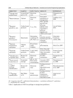
5.13 Industrial Applications
Some interesting applications of genetic programming in the industry are mentioned
here. In 2006 J.U. Dolinsky and others [9] presented a paper with an application of
genetic programming to the calibration of industrial robots. They state that most of
the proposed methods address the calibration problem by establishing models fol-
lowed by indirect and often ill-conditioned numeric parameter identification. They

proposed an inverse static kinematic calibration technique based on genetic pro-
gramming, used to establish and identify model parameters.
Another application is the use of genetic programming for drug discovery in
the pharmaceutical industry [10]. W.B. Langdon and S.K. Barrett employed genetic
programming while working in conjunction with GlaxoSmithKline (GSK). They
were invited to predict biochemical activity using their favorite machine learning
technique. Their genetic programming was the best of 12 tested, which marginally
improved the existing system of GSK.
5.14 Advantages of Evolutionary Algorithms
Probably the greatest advantage of evolutionary algorithms is their ability to address
problems for which there are no human experts. Although human expertise is to
be used when available, it has proven less than adequate for automating problem-
solving routines.
A primary advantage of this kind of algorithm is that they are simple to represent.
They can be modeled as a difference equation xŒtC 1 D s.r.xŒt//, which can
5.15 Genetic Programming Algorithm 145
be understood as: xŒtis the population at time t under the representation x,isthe
random variation operator and s is the selection operator.
The representation does not affect the p erformance of the algorithm, in contrast
with other numerical techniques, which are biased on continuous values or con-
strained sets. They offer a framework to easily incorporate known knowledge of
the problem, which could yield in a more efficient exploration and response of the
search space.
Evolutionary algorithms can be combined with simple or complex traditional
optimization techniques. Most of the time the solution can be evaluated in paral-
lel, and only the selection mu st be processed serially. This is an advantage over
other optimization techniques like tabu search and simulated annealing. Evolution-
ary algorithms can be used to adapt solutions to changing circumstances, because
traditional methods are not robust to dynamic changes and often require a restart to
provide the solution.

5.15 Genetic Programming Algorithm
In 1992, J.R. Koza developed a variation of GAs that is able to automate the gener-
ation of computer programs [8]. Evolutionary algorithms, also known as evolution-
ary computing, are the general principles of natural evolution that can be applied
to completely artificial enviro nments. GAs and genetic programming are types of
evolutionary computing.
Fig. 5.23 Tree representation
of a rule
146 5 Genetic Algorithms and Genetic Programming
Genetic programming is a computing method, which provides a system with the
possibility of generating optimized programs or computer codes. In genetic pro-
gramming IF-THEN rules are coded into individuals, which often are represented
as trees. For example, a rule for a wheeled robot may be IF left is far AND center if
far AND right is close THEN turn left. This rule is represented as a tree in Fig. 5.23.
According to W. Banzhaf “genetic programming, shall include systems that con-
stitute or contain explicit references to programs (executable code) or to program-
ming language expressions.”
5.15.1 Length
In GAs the length of the chromosome is fixed, which can restrict the algorithm to
a non-optimal region of the problem in search space. Because of the tree represen-
tation, genetic programming can create chromosomes of almost any length.
5.16 Genetic Programming Stages
Genetic programming uses four steps to solve problems:
1. Generate an initial population of random compositions of functions and termi-
nals of the problem (computer programs).
2. Execute each program in the population a nd assign it a fitness value according
to how well it solves the problem.
3. Create a new population of computer programs:
a. Copy the best existing programs.
b. Create new programs by mutation.

c. Create new computer programs by crossover.
4. The best computer program that appeared in any generation, the best-so-far so-
lution, is designated the result of genetic programming [8].
Just like in GAs, in genetic programming the stages are initialization, selection,
crossover, and mutation.
5.16.1 Initialization
There are two methods for creating the initial population in a genetic programming
system:
1. Full selects nodes from only the function set until a node is at a specified maxi-
mum depth.
2. Grow randomly selects nodes from the function and terminal set, which are
added to a new individual.
5.16 Genetic Programming Stages 147
5.16.2 Fitness
It could be the case that a function to be optimized is available, and we will just need
to program it. But for many problems it is not easy to define an objective function.
In such a case we may use a set of training examples and define the fitness as an
error-based function. These training examples should describe the behavior of the
system as a set of input/output relations.
Considering a training set of k examples we may have .x
i
;y
i
/; i D 1;:::;k;
where x
i
is the input of the ith training sample and y
i
is the corresponding output.
The set should be sufficiently large to provide a basis for evaluating programs over

a number of different significant situations.
The fitness functionmay also be defined as the total sum of squared errors; it has the
property of decreasing the importance of small deviations from the target outputs. If
we define the error as e
i
D .y
i
 o
i
/
2
where y
i
is the desired output and o
i
the actual
output, then the fitness will be defined as
P
k
iD1
e
k
D
P
k
iD1
.y
i
 o
i

/
2
. The fitness
function may also be scaled, thus allowing amplification of certain differences.
5.16.3 Selection
Selection operators within genetic programming are not specific; the problem under
consideration imposes a particular choice. The choice of the most appropriate selec-
tion operator is one of the most difficult problems, because generally this choice is
problem-dependent. However, the most-used method for selecting individuals in ge-
netic programming is tournament selection, because it does not require a centralized
fitness comparison between all individuals. The best individuals of the generation
are selected.
5.16.4 Crossover
The form of the recombination operators depends on the representation of individu-
als, but we will restrict ourselves to tree-structured representations. An elegant and
rather straightforward recombination operator acting o n two parents swaps a subtree
of one parent with a subtree of the other parent.
There is a method proposed by H. Iba and H. Garis to detect regularities in
the tree program structure and to use them as guidance for the crossover opera-
tor. The method assigns a performance value to a subtree, which is used to select
the crossover points. Thus, the crossover operator learns to choose good sites for
crossover.
Simple crossover operation. In a random position two trees interchange their
branches, but it should be in a way such that syntactic correctness is maintained.
Each offspring individual will pass to the selection process of the next generation.
In Fig. 5.24 a representation of a crossover is shown.
148 5 Genetic Algorithms and Genetic Programming
Fig. 5.24 Tree representation of a genetic programming crossover stage
5.16.5 Mutation
There are several mutation techniques proposed for genetic programming. An ex-

ample is the mutation of tree-structured programs; here the mutation is applied to
a single program tree to generate an offspring. If our program is linearly repre-
5.17 Variations of Genetic Programming 149
Fig. 5.25 Tree representation of a genetic programming mutation stage
sented, then the mutation operator selects an instruction from the individual chosen
for mutation. Then, this selected instruction is randomly perturbed, or is changed to
another instruction randomly chosen from a pool of instructions.
The usual strategy is to complete the offspring population with a crossover op-
eration. On this kind of population the mutation is applied with a specific mutation
probability. A different strategy considers a separate application of cro ssover and
mutation. In this case it seems to be emphasized with respect to the previous, stan-
dard technology.
In genetic programming, the generated individuals are selected with a very low
probability of being mutated. When an individual is mutated, one of its nodes is se-
lected randomly and then the current subtree at that point is replaced with a new ran-
domly generated subtree. It is important to state that just as in biological mutation,
in genetic programming mutation the genotype may not change but the resulting
genotype could be completely different (Fig. 5.25).
5.17 Variations of Genetic Programming
Several variations of genetic programming can be found in the literature. Some of
them are linear genetic programming, a variant that acts o n linear genomes rather
than trees; gene expression programming, where the genotype (a linear chromo-
some) and the phenotype (expression trees) are different entities that form an indi-
visible whole; multi-expression programming encodes several solutions into a chro-
mosome; Cartesian genetic programming uses a network of nodes (indexed graph)
to achieve an input-to-output mapping; and traceless genetic programming, which
does not store explicitly the evolved com puter programs, and is useful when the
relation between the input and output is not important.
150 5 Genetic Algorithms and Genetic Programming
5.18 Genetic Programming in Data Modeling

The main purpose of evolutionary algorithms is to imitate natural selection and evo-
lution, allowing the most efficient individuals to reproduce more often. Genetic pro-
gramming is very similar to GAs; the main difference is that genetic programming
uses different coding of potential solutions. By using knowledge from great amounts
of data collected from different places, we can discover patterns and represent them
in a way that humans can understand them.
By mathematical modeling we understand that certain equations fit some nu-
merical data. It is used in a variety o f scientific problems, where the theoretical
foundations are not enough to give answers to experiments. Sometimes using tra-
ditional methods is not enough because these m ethods assume a specific form of
model. Genetic programming allows the search for a good model in a different and
more “intelligent” way, and can be used to solve highly complex, non-linear, chaotic
problems.
5.19 Genetic Programming Using the ICTL
Here we will continue with the optimization example of fuzzy systems. As we have
mentioned previously, a Takagi–Sugeno is the core controller of a navigation system
that maneuvers the movements of a quadruped robot in order to avoid obstacles. We
have previously optimized the form of the membership functions using GAs and
now we will evolve the form o f the rules and modify their operators. The rules for
the controllers used in the quadruped robot have the form of (5.4):
IF Left is ALi Conn Central is ACi Conn Right is ARi THEN SLeft, SRight ;
(5.4)
where ALi D AC i D AR i are the number of fuzzifying membership functions for
the inputs, in this case they are the same, and Conn is the operation to be performed.
There are four options: (1) min,(2)max,(3)product,and(4)sum. SLeft, SRight are
the speeds used to control the movements of the robot.
Genetic programming will be applied using the following convention to code-
decode the individuals:
• 3 bits that will help us determine if the set is complemented or not. A bi-
dimensional array must be generated with the same form of the CM-A of the

input-combinator-generator.vi that is used to evaluate the different sets of the
possible rule combinations. The first dimension contains the number of rules, the
second the number of inputs to the system.
• 2 bits are used for the premise evaluation. The premises of the next connection
operation are used: (0) min,(1)max,(2)product,and(3)sum.
• 10 bits are used to obtain the outputs of the rule, 5 for each output to obtain
a constant between 0 and 31.
5.19 Genetic Programming Using the ICTL 151
Tabl e 5.4 Individual rule coding for genetic programming ICTL example
Three bits Two bits 10 bits for rule output
IS, IS NOT Conn
01234567891011121314
Fig. 5.26 Localization of genetic programming methods on the ICTL
The rule in bits is shown in Table 5.4. As shown in Fig. 5.26, the methods for genetic
programming are found at Optimizers  GPs  Generic Methods. An individual
contains 27 of these rules; the initial_population.vi initializes a population with
random individuals. The code is shown in Fig. 5.27. Fixed individuals may be added
based on human expert knowledge.
Fig. 5.27 Block diagram for
the initialization of random
individuals
Fig. 5.28 Block diagram of fitness function
152 5 Genetic Algorithms and Genetic Programming
Fig. 5.29 Front panel of the genetic programming e xample
Fig. 5.30 Block diagram of the genetic programming example
The fitness function (Figs. 5.28–5.30) compares a series of desired inputs and
outputs with the corresponding performance of the controller, calculating the quadra-
tic errors difference with each point, summing them and dividing by the number of
evaluated points to obtain the fitness value for a given individual.
The selection function executes the tournament variation by randomly selecting

a d esired number of individuals and selecting the two fittest. This process is repeated
until the same number of initial individuals is obtained.
References 153
Tabl e 5.5 Controlled variables in the genetic programming example
Variable Description
Pop Size The number of indi viduals in the algorithm.
IinT The number of individuals randomly taken for the tournament selection.
Cr Prob The probability of crossing [0, 1].
Mt Prob The probability of mutation for each bit [0, 1].
The crossover executes a one-stage interchange of tails, by taking two individ-
uals from the mating pool, and depending on the possibility of crossing, the two
individuals will or will not perform the crossover again. This process is repeated
until the same number of initial individuals is obtained.
The mutation process executes a bit-to-bit operation on every one of the rules of
each individual, and depending on the probability of mutation the bit will or will not
change. During the execution of this algorithm, the individual with the best fitness
is always stored to ensure that this information is never lost. Table 5.5 shows the
variables to be controlled.
References
1. Wang F, et al. (2006) Design optimization of industrial motor drive po wer stage using ge-
netic algorithms. Proceedings of CES/IEEE 5th I nternational Power Electronics and Motion
Control Conference (IPEMC), 1–5 Aug 2006, vol 1, pp 14–16
2. Cho D-H, et al. (2001) Induction motor design of electric vehicle using a niching genetic
algorithm. IEEE Trans I nd Appl USA 37(4):994–999
3. Cav alieri S ( 1999) A genetic algorithm for job-shop scheduling in a semiconductor manufac-
turing system. Proceedings of the 25th Annual Conference of the IEEE on Industrial Electron-
ics Society (IECON) 1999, Italy, 29 Nov to 3 Dec 1999, vol 2, pp 957–961
4. Colla V, et al. (1998) Model parameter optimization for an industrial application: a comparison
between traditional and genetic algorithms. Proceedings of the IEEE 2nd UKSIM European
Symposium on Computer Modeling and Simulation, 8–10 Sept 2008, pp 34–39

5. Haupt RL, Haupt SE (1998) Practical genetic algorithms. W iley-Interscience, New York
6. Mitchell M (1998) An introduction to genetic algorithms. MIT Press, Cambridge, MA
7. Cramer NL (1985) A representation for the adaptive generation of simple sequential pro-
grams. In: Grefenstette JJ (ed) Proceedings of the First International Conference on Genetic
Algorithms and T heir Applications. Erlbaum, Mahwah, NJ
8. Koza JR (1992) Genetic programming: on the programming of computers by means of natural
selection. MIT Press, Cambridge, MA
9. Dolinsky JU, et al. (2007) Application of genetic programming to the calibrating of industrial
robots. ScienceDirect Comput Ind 58(3):255–264
10. Langdon WB, Buxton BF (2003) The application of genetic programming for drug disco very
in the pharmaceutical industry. EPSRC RIAS project with GlaxoSmithKline. London, UK,
September 2003
154 5 Genetic Algorithms and Genetic Programming
Futher Reading
Dumitrescu D, et al. (2000) Evolutionary computation. CRC, Boca Raton, FL
Ghanea-Hercock R (2003) Applied evolutionary algorithms in Java. Springer, Berlin Heidelberg
New York
Nedjah N, et al. (2006) Genetic systems programming theory and experiences. Springer, Berlin
Heidelberg New York
Reeves CR, Rowe JE (2004) Genetic algorithms principles and perspectives: A guide to GA theory.
Kluwer, Dordrecht
Chapter 6
Simulated Annealing, FCM,
Partition Coefficients and Tabu Search
6.1 Introduction
In 1945 the construction of the first computer caused a revolution in the world. It
was aimed to modify the interactions between Russia and the West. In the academic
and research fields it brought back a mathematical technique known as statistical
sampling, now referred to as the Monte Carlo method. S. Frankel and N. Metropolis
created a model of a thermonuclear reaction for the Electronic Numerical Integra-

tor and Computer (ENIAC), persuaded by the curiosity and interest of John von
Neumann, a prominent scientist in that field.
The results of the model where obtained after the end of the World War I, and
among the reviewers was Stan Ulam, who had an extensive background in mathe-
matics and the use of statistical methods. He knew these techniques were no longer
in use because of the length and tediousness of calculations. His research interest
included pattern development in 2 D games played with very simple rules. These
techniques are now used in various industrial applications known as cellular au-
tomata.
Ulam and Neumann sent a proposal of the Monte Carlo method to the theoret-
ical division leader of the Los Alamos Laboratory in New Mexico in 1947, which
included a detailed outline of a possible statistical approach to solve the problem
of neutron diffusion in fissionable material. The basic idea of the method was to
generate a genealogical history of different variables in a pr ocess until a statistically
valid picture of each variable was created.
The next step was to generate random numbers; here Neumann proposed a method
called the middle-square digits. Once the random numbers are generated, they must
be transformed into a non-uniform distribution desired for the property of interest.
Solving problems using this method is easier than other ap proaches like differen-
tial equations, because one needs only to mirror the probability distribution in to the
search space of the problem at hand.
In 1947 the ENIAC was moved to the Ballistic Research Laboratory in Maryland,
its permanent home. After the movement, there was an explosion in the use of the
P. Ponce-Cruz, F. D. Ramirez-Figueroa, Intelligent Control Systems with LabVIEW™ 155
© Springer 2010
156 6 Simulated Annealing, FCM, Partition Coefficients and Tabu Search
Monte Carlo method with this computer. The applications solved several questions
of different branches of physics, and by 1949 there was a special symposium held
on the method.
The Monte Carlo method gave birth to modern computational optimization prob-

lems. We can now see, as a natural consequence of electronic computers, the quick
evolution of experimental mathematics, with th e Monte Carlo method key to this
achievement. It was at this point that mathematics achieved the twofold aspect of
experiment and theory, which all other sciences enjoy.
As an example of the method, we can imagine a coconut shy. We want to know
the probability of taking 10 shots at the coconut shy and obtain an even number of
hits. The only information that we know is that there is a 0.2 probability of having
a hit with a single shot. Using the Monte Carlo method we can perform a large
number of simulations of taking 10 shots at the coconut shy. Next we can count the
simulations with even number of hits and divide that number over the total number
of simulations. By doing this we will get an approximation of the probability that
we are looking for.
6.1.1 Introduction to Simulated Annealing
A combinatorial optimization problem strives to find the best or optimal solution,
among a finite or infinite number of solutions. A wide variety of combinatorial prob-
lems have emerged from different areas such as physical sciences, computer science,
and engineering, among others. Considerable effort has been devoted to construct
and research methods for solving the performance of the techniques. Integer, linear,
and non-linear programming have been the major breakthroughs in recent times.
Over the years it has been shown that many theoretical and p ractical problems
belong to the class of NP-complete p roblems. A large number of these problems
are still unsolved ; there are two main options for solving them. On the one hand,
if we strive for optimality the computation time will be very large; these methods
are called optimization methods. On the other hand, we can search quick solutions
with suboptimal performance, called heuristic algorithms. However, the difference
between these methods is not very strict, because some types of algorithm can be
used for both purposes.
Another way to classify algorithms is between general and tailored. While gen-
eral algorithms are applicable to a wide range of problems, tailored algorithms use
problem-specific information, restricting their applicab ility. The intrinsic problem

is that for the former ones, for each type of combinatorial optimization problem,
a new algorithm must be constructed.
6.1 Introduction 157
6.1.2 Pattern Recognition
Recognizing and classifying patterns is a fundamental characteristic of human intel-
ligence. It plays a key role in human perceptio n as well as other levels of cognition.
The field of study has evolved since the 1950s. Pattern recognition can be defined
as a process by which we search for structures in data and classify them into cate-
gories such that the degree of association is high among structures of the same kind.
Prototypical categories are usually characterized from past experience, and can be
done by more than one structure.
Classification of objects falls in the category of cluster analysis, which plays
a key role in pattern recognition. Cluster analysis it is not restricted to only pattern
recognition, but is applicable to the taxonomies in biology and other areas, classifi-
cation of information, and social groupings.
Fuzzy set theory has been used in pattern recognition since the mid-1960s. We
can find three fundamental problems in pattern recognition, where most categories
have vague boundaries. In general, objects are represented by a vector of measured
values of r variables: a D Œa
1
:::a
r
.
This vector is called a pattern vector, where a
i
(for each i 2 N
r
/ is a particu -
lar characteristic of interest. The first problem is concerned with representation of
input data, which is obtained from the objects to be recognized, known as sensing

problems. The second problem concerns the extraction of different features from the
input data, in terms of the dimension of the pattern vector; they are called feature
extraction problems. These features should characterize attributes, which determine
the pattern classes.
The third problem involves the determination of optimal decision procedures for
the classification of given patterns. Most of the time this is done by defining an ap-
propriate discrimination function of patterns by assigning a real number to a pattern
vector. Then, individual pattern vectors are evaluated by discrimination functions,
and the classification is designed by the resulting number.
6.1.3 Introduction to Tabu Search
There are many problems that n eed to be solved by optimization p rocedures. Ge-
netic algorithms (GA) or simulated annealing is used for that purpose. Tabu search
(TS) is among the methods found in this field of optimization solutions. As its name
suggests, tabu search is an algorithm performing the search in a region for the min-
imum or maximum solution of a given problem.
Searching is quite complicated because it uses a lot of memory and spends too
much time in th e process. For this reason, tabu search is implem ented as an intelli-
gent algorithm to take advantage of memory and to search more efficiently.
158 6 Simulated Annealing, FCM, Partition Coefficients and Tabu Search
6.1.4 Industrial Applications of Simulated Annealing
We will briefly describe some industrial applications of the simulated annealing.
Scheduling is always a difficult problem in the industry. Processes and logistics
must be carefully combined to harmonize and increase production of plants. In 1997
A.P. Reynolds [1] and others presented a paper on simulated annealing for indus-
trial applications. They optim ized the scheduling process in order to optimize the
resources of a manufacturing plant to meet the demand of different products.
S. Saika and other researchers [2] from Matsushita at the Advanced LSI Tech-
nology Development Center introduced a high-performance simulated annealing
application to transistor placement. Called widely stepping simulated annealing,
they applied it to the 1D transistor placement optimizations used in several in-

dustrial cells. They claim to have solutions as good as the standard algorithm
and better, with a processing time one-thirtieth that of the normal simulated an-
nealing.
R.N. Bailey, K.M. Garner, and M.F. Hobbs published a paper [3] showing the
application of simulated annealing and GAs to solve staff scheduling problems.
They use the algorithms to solve the scheduling of the work of staff with different
skill levels, which is difficult to achieve because there is a large number of solu-
tions. The results show that both simulated annealing and GAs can produce opti-
mal and near-optimal solutions in a relatively short time for the nurse scheduling
problem.
6.1.5 Industrial Applications of Fuzzy Clustering
Manufacturing firms have increased the use of industrial robots over the years. There
has also been an increase in the number of robot manufacturers, offering a wide
range of products. This is how M. Khouja and D.E. Booth [4] used a fuzzy cluster-
ing technique for the evaluation and selection of industrial robots given a specific
application. They take in to consideration real-world data instead to create the model.
B. Moshiri and S. Chaychi [5] use fuzzy logic and fuzzy clustering to model
complex systems and identify non-linear industrial processes. They claim that their
proposed advantage is simple, flexible and of high accuracy, easy to use and auto-
matic. They applied this system to a heat exchanger.
6.1.6 Industrial Applications of Tabu Search
Tabu search has been widely used to optimize several industrial applications. For
example, L. Zhang [6] and his team proposed a tabu search scheme to optimize the
vehicle routing problem, with the objective of finding a schedule that will guarantee
6.2 Simulated Annealing 159
the safety of all vehicles. Their algorithm proved to be good enough compared with
other more mature algorithms specially designed for the vehicle problem.
Artificial neural network s (ANNs) based on the tabu search algorithm have also
been used by H. Shuang [7] to create a wind speed prediction model. A backpropa-
gation neural network has its weights optimized using tabu search. Then the neural

network is used as a model to predict the wind speed 1 hour ahead. It improved the
prediction compared with a simple backpropagation neural network.
In 2007 J. Brigitte and S. Sebbah presented a paper [8] in which 3G networks
are optimized. The location of primary bases and the core network link capacity is
optimized. The dimensioning problem is modeled as a mixed-integer program and
solved by a tabu search algorithm; the search criteria includes the signal-to-noise
plus interference ratio. Primary bases are randomly located and after a few iterations
their location is changed and the dimensioning optimized.
This base optimization problem was previously addressed by C.Y. Lee and pub-
lished in a paper in 2000 [9]. He also aimed to minimize the number of base stations
used and its location in an area covered by cellular communications. The results
presented show that a 10 % in cost reduction is achieved, and between a 10 and 20%
of cost reduction in problems with 2500 traffic demand areas with code division
multiple access (CDMA) systems.
6.2 Simulated Annealing
It was in 1982 and 1983 that Kirkpatrick, Gelatt and Vecchi introduced the concepts
of annealing in combinatorial optimization. It was also independently presented in
1985 by
ˇ
Cerny. The concepts are based on the physical annealing process of solids
and the problem of solving large optimization problems.
Annealing is a physical process where a substance is heated and cooled in a con-
trolled manner. The results obtained by this process are strong crystalline structures,
compared to structures obtained by fast untempered cooling, which result in brittle
and defective structures. For the optimization process the structure is our encoded
solution, and the temperature is used to determine how and when new solutions are
accepted. The process contains two steps [4, 10]:
1. Increase temperature of the heat ba th to a maximum value at which the solid
melts.
2. Carefully decrease the temperature of the heat bath until particles arrange them-

selves in the g round state of the solid.
When the structure is in the liquid phase all the particles of the solid arrange them-
selves in a random way. In the ground state the particles are arranged in a highly
structured lattice, leaving the energy of the system at its minimum. This ground state
of the solid is only obtained if the maximum temperature is sufficiently high and the
cooling is sufficiently low, otherwise, the solid will be frozen into a metastable state
rather than the ground state.