Dynamic Speech ModelsTheory, Algorithms, and Applications phần 9 ppsx
Bạn đang xem bản rút gọn của tài liệu. Xem và tải ngay bản đầy đủ của tài liệu tại đây (905.03 KB, 11 trang )
P1: IML/FFX P2: IML
MOBK024-05 MOBK024-LiDeng.cls April 26, 2006 14:3
MODELS WITH CONTINUOUS-VALUED HIDDEN SPEECH TRAJECTORIES 83
Frame (10 ms)
Frequency (kHz)
γ = [0.6],
D
= 7
0 20 40 60 80 100 120 140 160 180 200
0
1
2
3
4
5
6
FIGURE 5.8: Same as Fig. 5.7 except with another utterance “Be excited and don’t identify yourself ”
(SI1669)
the three example TIMIT utterances. Note that the model prediction includes residual means,
which are trained from the full TIMIT data set using an HTK tool. The zero-mean random
component of the residual is ignored in these figures. The residual means for the substates
(three for each phone) are added sequentially to the output of the nonlinear function Eq. (5.12),
assuming each substate occupies three equal-length subsegments of the entire phone segment
length provided by TIMIT database. To avoid display cluttering, only linear cepstra with orders
one (C1), two (C2) and three (C3) are shown here, as the solid lines. Dashed lines are the linear
cepstral data C1, C2 and C3 computed directly from the waveforms of the same utterances
for comparison purposes. The data and the model prediction generally agree with each other,
somewhat better for lowerorder cepstra than for higherorder ones. It was found that these
discrepancies are generally within the variances of the prediction residuals automatically trained
from the entire TIMIT training set (using an HTK tool for monophone HMM training).
P1: IML/FFX P2: IML
MOBK024-05 MOBK024-LiDeng.cls April 26, 2006 14:3
84 DYNAMIC SPEECH MODELS
Frame (10 ms)
Frequency (kHz)
γ = [0.6],
D
= 7
0 50 100 150 200 250
0
1
2
3
4
5
6
FIGURE 5.9: Same as Fig. 5.7 except with the third utterance “Sometimes, he coincided with my father’s
being at home ” (SI2299)
5.3 PARAMETER ESTIMATION
In this section, we will present in detail a novel parameter estimation algorithm we have devel-
oped and implemented for the HTM described in the preceding section, using the linear cepstra
as the acoustic observation data in the training set. The criterion used for this training is to
maximize the acoustic observation likelihood in Eq. (5.20). The full set of the HTM parameters
consists of those characterizing the linear cepstra residual distributions and those characterizing
the VTR target distributions. We present their estimation separately below, assuming that all
phone boundaries are given (as in the TIMIT training data set).
5.3.1 Cepstral Residuals’ Distributional Parameters
This subset of the HTM parameters consists of (1) the mean vectors μ
r
s
and (2) the diagonal
elements σ
2
r
s
in the covariance matrices of the cepstral prediction residuals. Both of them are
conditioned on phone or sub-phone segmental unit s .
P1: IML/FFX P2: IML
MOBK024-05 MOBK024-LiDeng.cls April 26, 2006 14:3
MODELS WITH CONTINUOUS-VALUED HIDDEN SPEECH TRAJECTORIES 85
0 50 100 150 200 250 300 350
0 50 100 150 200 250 300 350
0 50 100 150 200 250 300 350
−1
0
1
−0.5
0
0.5
−2
−1
0
1
2
Frame (10 ms)
C1
C2
C3
FIGURE 5.10: Linear cepstra with order one (C1), two (C2) and three (C3) predicted from the final
stage of the model generating the linear cepstra (solid lines) with the input from the FIR filtered results
(for utterance SI1039). Dashed lines are the linear cepstral data C1, C2 and C3 computed directly from
the waveform
Mean Vectors
To find the ML (maximum likelihood) estimate of parameters μ
r
s
,weset
∂ log
K
k=1
p(o(k) |s)
∂μ
r
s
= 0,
where p(o(k) |s ) is given by Eq. (5.20), and K denotes the total duration of sub-phone s in the
training data. This gives
K
k=1
o(k) −
¯
μ
o
s
= 0, or (5.23)
P1: IML/FFX P2: IML
MOBK024-05 MOBK024-LiDeng.cls April 26, 2006 14:3
86 DYNAMIC SPEECH MODELS
0 20 40 60 80 100 120 140 160 180 200
−1
−0.5
0
0.5
0 20 40 60 80 100 120 140 160 180 200
−0.5
0
0.5
0 20 40 60 80 100 120 140 160 180 200
−2
−1
0
1
2
Frame (10 ms)
C1
C2
C3
FIGURE 5.11: Same as Fig. 5.10 except with the second utterance (SI2299)
K
k=1
o(k) −F
[z
0
(k)]μ
z
(k)
−{F[z
0
(k)] + μ
r
s
− F
[z
0
(k)]z
0
(k)}
= 0. (5.24)
Solving for μ
r
s
, we have the estimation formula of
ˆ
μ
r
s
=
k
o(k) −F[z
0
(k)] − F
[z
0
(k)]μ
z
(k) + F
[z
0
(k)]z
0
(k)
K
. (5.25)
Diagonal Covariance Matrices
Denote the diagonal elements of the covariance matrices for the residuals as a vector σ
2
r
s
.To
derive the ML estimate, we set
∂ log
K
k=1
p(o(k) |s)
∂σ
2
r
s
= 0,
P1: IML/FFX P2: IML
MOBK024-05 MOBK024-LiDeng.cls April 26, 2006 14:3
MODELS WITH CONTINUOUS-VALUED HIDDEN SPEECH TRAJECTORIES 87
0 50 100 150 200 250
−1
−0.5
0
0.5
0 50 100 150 200 250
−0.5
0
0.5
0 50 100 150 200 250
−2
−1
0
1
2
Frame (10 ms)
C1
C2
C3
FIGURE 5.12: Same as Fig. 5.10 except with the third utterance (SI1669)
which gives
K
k=1
σ
2
r
s
+ q(k) −(o(k) −
¯
μ
o
s
)
2
[σ
2
r
s
+ q(k)]
2
= 0, (5.26)
where vector squaring is the element-wise operation, and
q(k) = diag
F
[z
0
(k)]Σ
z
(k)(F
[z
0
(k)])
Tr
. (5.27)
Due to the frame (k) dependency in the denominator in Eq. (5.26), no simple closed-form
solution is available for solving σ
2
r
s
from Eq. (5.26). We have implemented three different
techniques for seeking approximate ML estimates that are outlined as follows:
1. Frame-independent approximation: Assume the dependency of q(k) on time frame k is
mild, or q(k) ≈
¯
q. Then the denominator in Eq. (5.26) can be cancelled, yielding the
P1: IML/FFX P2: IML
MOBK024-05 MOBK024-LiDeng.cls April 26, 2006 14:3
88 DYNAMIC SPEECH MODELS
approximate closed-form estimate of
ˆ
σ
2
r
s
≈
K
k=1
(o(k) −
¯
μ
o
s
)
2
− q(k)
K
. (5.28)
2. Direct gradient ascent: Make no assumption of the above, and take the left-hand side of
Eq. (5.26) as the gradient ∇L of log-likelihood of the data in the standard gradient-
ascent algorithm:
σ
2
r
s
(t + 1) = σ
2
r
s
(t) +
t
∇L(o
K
1
|σ
2
r
s
(t)),
where
t
is a heuristically chosen positive constant controlling the learning rate at the
t-th iteration.
3. Constrained gradient ascent: Add to the previous standard gradient ascent technique the
constraint that the variance estimate be always positive. The constraint is established
by the parameter transformation:
˜
σ
2
r
s
= log σ
2
r
s
, and by performing gradient ascent for
˜
σ
2
r
s
instead for σ
2
r
s
:
˜
σ
2
r
s
(t + 1) =
˜
σ
2
r
s
(t) +
˜
t
∇
˜
L(o
K
1
|
˜
σ
2
r
s
(t)),
Using chain rule, we show below that the new gradient ∇
˜
L is related to the gradient
∇L before parameter transformation in a simple manner:
∇
˜
L =
∂
˜
L
∂
˜
σ
2
r
s
=
∂
˜
L
∂σ
2
r
s
∂σ
2
r
s
∂
˜
σ
2
r
s
= (∇L) exp(
˜
σ
2
r
s
).
Attheendof thealgorithmiteration,the parametersaretransformedviaσ
2
r
s
= exp(
˜
σ
2
r
s
),
which is guaranteed to be positive.
For efficiency purposes, parameter updating in the above gradient ascent techniques is
carried out after each utterance in the training, rather than after the entire batch of all utterances.
We note that the quality of the estimates for the residual parameters discussed above plays
a crucial role in phonetic recognition performance. These parameters provide an important
mechanism for distinguishing speech sounds that belong to different manners of articulation.
This is attributed to the fact that nonlinear cepstral prediction from VTRs has different accuracy
for these different classes of sounds. Within the same manner class, the phonetic separation
is largely accomplished by distinct VTR targets, which typically induce significantly different
cepstral prediction values via the “amplification” mechanism provided by the Jacobian matrix
F
[z].
P1: IML/FFX P2: IML
MOBK024-05 MOBK024-LiDeng.cls April 26, 2006 14:3
MODELS WITH CONTINUOUS-VALUED HIDDEN SPEECH TRAJECTORIES 89
5.3.2 Vocal Tract Resonance Targets’ Distributional Parameters
This subset of the HTM parameters consists of (1) the mean vectors μ
T
s
and (2) the diagonal
elements σ
2
T
s
in the covariance matrices of the stochastic segmental VTR targets. They are also
conditioned on phone segment s (and not on sub-phone segment).
Mean Vectors
To obtain a closed-form estimation solution, we assume diagonality of the prediction cepstral
residual’s covariance matrix Σ
r
s
. Denoting its qth component by σ
2
r
(q)(q = 1, 2, ,Q), we
decompose the multivariate Gaussian of Eq. (5.20) element-by-element into
p(o(k) |s(k)) =
J
j=1
1
2πσ
2
o
s (k)
( j)
exp
−
(o
k
( j) −
¯
μ
o
s (k)
( j))
2
2σ
2
o
s (k)
( j)
, (5.29)
where o
k
( j) denotes the jth component (i.e., jth order) of the cepstral observation vector at
frame k.
The log-likelihood function for a training data sequence (k = 1, 2, ,K) relevant to
the VTR mean vector μ
T
s
becomes
P =
K
k=1
J
j=1
−
(o
k
( j) −
¯
μ
o
s (k)
( j))
2
σ
2
o
s (k)
( j)
(5.30)
=
K
k=1
J
j=1
[
f
F
[z
0
(k), j, f ]
l
a
k
(l)μ
T
(l, f ) − d
k
( j)]
2
σ
2
o
s (k)
( j)
,
where l and f are indices to phone and to VTR component, respectively, and
d
k
( j) = o
k
( j) − F[z
0
(k), j] +
f
F
[z
0
(k), j, f ]z
0
(k, f ) − μ
r
s (k)
( j).
While the acoustic feature’s distribution is Gaussian for both HTM and HMM given
the state s , the key difference is that the mean and variance in HTM as in Eq. (5.20) are both
time-varying functions (hence trajectory model). These functions provide context dependency
(and possible target undershooting) via the smoothing of targets across phonetic units in the
utterance. This smoothing is explicitly represented in the weighted sum over all phones in the
utterance (i.e.,
l
) in Eq. (5.30).
Setting
∂P
∂μ
T
(l
0
, f
0
)
= 0,
P1: IML/FFX P2: IML
MOBK024-05 MOBK024-LiDeng.cls April 26, 2006 14:3
90 DYNAMIC SPEECH MODELS
and grouping terms involving unknown μ
T
(l, f ) on the left and the remaining terms on the
right, we obtain
f
l
A(l, f ;l
0
, f
0
)μ
T
(l, f )
=
k
j
F
[z
0
(k), j, f
0
]
σ
2
o
s (k)
( j)
d
k
( j)
a
k
(l
0
), (5.31)
with f
0
= 1, 2, ,8 for each VTR dimension, and with l
0
= 1, 2, ,58 for each phone unit.
In Eq. (5.31),
A(l, f ;l
0
, f
0
) =
k, j
F
[z
0
(k), j, f ]F
[z
0
(k), j, f
0
]
σ
2
o
s (k)
( j)
a
k
(l
0
)a
k
(l). (5.32)
Eq. (5.31) is a 464 × 464 full-rank linear system of equations. (The dimension 464 =
58 × 8 where we have a total of 58 phones in the TIMIT database after decomposing each
diphthong into two “phones”, and 8 is the VTR vector dimension.) Matrix inversion gives an
ML estimate of the complete set of target mean parameters: a 464-dimensional vector formed
by concatenating all eight VTR components (four frequencies and four bandwidths) of the
58 phone units in TIMIT.
In implementing Eq. (5.31) for the ML solution to target mean vectors, we kept other
model parameters constant. Estimation of the target and residual parameters was carried out
in an iterative manner. Initialization of the parameters μ
T
(l, f ) was provided by the values
described in [9].
An alternative training of the target mean parameters in a simplified version of the HTM
and its experimental evaluation are described in [112]. In that training, the VTR tracking
results obtained by the tracking algorithm described in Chapter 4 are exploited as the basis for
learning, contrasting the learning described in this section, which uses the raw cepstral acoustic
data only. Use of the VTR tracking results enables speaker-adaptive learning for the VTR target
parameters as shown in [112].
Diagonal Covariance Matrices
To establish the objective function for optimization, we take logarithm on the sum of the
likelihood function Eq. (5.29) (over K frames) to obtain
L
T
∝−
K
k=1
J
j=1
(o
k
( j) −
¯
μ
o
s (k)
( j))
2
σ
2
r
s
( j) + q(k, j)
+ log [σ
2
r
s
( j) + q(k, j)]
, (5.33)
P1: IML/FFX P2: IML
MOBK024-05 MOBK024-LiDeng.cls April 26, 2006 14:3
MODELS WITH CONTINUOUS-VALUED HIDDEN SPEECH TRAJECTORIES 91
where q(k, j)isthe jth element of the vector q(k) as defined in Eq. (5.27). When Σ
z
(k)is
diagonal, it can be shown that
q(k, j) =
f
σ
2
z(k)
( f )(F
jf
)
2
=
f
l
v
k
(l)σ
2
T
(l, f )(F
jf
)
2
, (5.34)
where F
jf
is the (j, f ) element of Jacobian matrix F
[·] in Eq. (5.27), and the second equality
is due to Eq. (5.11).
Using chain rule to compute the gradient, we obtain
∇L
T
(l, f ) =
∂ L
T
∂σ
2
T
(l, f )
(5.35)
=
K
k=1
J
j=1
(o
k
( j) −
¯
μ
o
s (k)
( j))
2
(F
jf
)
2
v
k
(l)
[σ
2
r
s
( j) + q(k, j)]
2
−
(F
jf
)
2
v
k
(l)
σ
2
r
s
( j) + q(k, j)
.
Gradient-ascend iterations then proceed as follows:
σ
2
T
(l, f ) ← σ
2
T
(l, f ) + ∇L
T
(l, f ),
for each phone l and for each element f in the diagonal VTR target covariance matrix.
5.4 APPLICATION TO PHONETIC RECOGNITION
5.4.1 Experimental Design
Phonetic recognition experiments have been conducted [124] aimed at evaluating the HTM
and the parameter learning algorithms described in this chapter. The standard TIMIT phone
set with 48 labels is expanded to 58 (as described in [9]) in training the HTM parameters using
the standard training utterances. Phonetic recognition errors are tabulated using the commonly
adopted 39 labels after the label folding. The results are reported on the standard core test set
of 192 utterances by 24 speakers [127].
Due to the high implementation and computational complexity for the full-fledged HTM
decoder, the experiments reported in [124] have been restricted to those obtained by N-best
rescoring and lattice-constrainedsearch. For each of the coretestutterances,astandarddecision-
tree-based triphone HMM with the bi-gram language model is used to generate a large N-best
list (N = 1000) and a large lattice. These N-best lists and lattices are used for the rescoring
experiments with the HTM. The HTM system is trained using the parameter estimation
algorithms described earlier in this chapter. Learning rates in the gradient ascent techniques
have been tuned empirically.
P1: IML/FFX P2: IML
MOBK024-05 MOBK024-LiDeng.cls April 26, 2006 14:3
92 DYNAMIC SPEECH MODELS
5.4.2 Experimental Results
In Table 5.1, phonetic recognition performance comparisons are shown between the HMM
system described above and three evaluation versions of the HTM system. The HTM-1 version
uses theHTM likelihoodcomputedfromEq.(5.20)torescore the1000-bestlists,and no HMM
score and language model (LM) score attached in the 1000-best list are exploited. The HTM-2
version improves the HTM-1 version slightly by linearly weighting the log-likelihoods of the
HTM, the HMM and the (bigram) LM, based on the same 1000-best lists. The HTM-3
version replaces the 1000-best lists by the lattices, and carries out A* search, constrained by the
lattices and with linearly weighted HTM–HMM–LM scores, to decode phonetic sequences.
(See a detailed technical description of this A*-based search algorithm in [111].) Notable
performance improvement is obtained as shown in the final row of Table 5.1. For all the
systems, the performance is measured by percent phone recognition accuracy (i.e., including
insertion errors) averaged over the core test-set sentences (numbers in bolds in column 2). The
percent-correctness performance (i.e., excluding insertion errors) is listed in column 3. The
substitution, deletion and insertion error rates are shown in the remaining columns.
The performance results in Table 5.1 are obtained using the identical acoustic features of
frequency-warped linear cepstra for all the systems. Frequency warping of linear cepstra [128]
has been implemented by a linear matrix-multiplication technique on both acoustic features and
the observation-prediction component of the HTM. The warping gives slight performance
improvement for both HMM and HTM systems by a similar amount. Overall, the lattice-
based HTM system (75.07% accuracy) gives 13% fewer errors than does the HMM system
TABLE5.1: TIMIT PhoneticRecognition PerformanceComparisonsBetween
an HMM System and Three Versions of the HTM System
ACC % CORR % SUB % DEL % INS %
HMM 71.43 73.64 17.14 9.22 2.21
HTM-1 74.31 77.76 16.23 6.01 3.45
HTM-2 74.59 77.73 15.61 6.65 3.14
HTM-3 75.07 78.28 15.94 5.78 3.20
Note. HTM-1: N-best rescoring with HTM scores only; HTM-2: N-
best rescoring with weighted HTM, HMM and LM scores; HTM-3:
Lattice-constrained A* search with weighted HTM, HMM and LM
scores. Identical acoustic features (frequency-warped linear cepstra) are
used.
P1: IML/FFX P2: IML
MOBK024-05 MOBK024-LiDeng.cls April 26, 2006 14:3
MODELS WITH CONTINUOUS-VALUED HIDDEN SPEECH TRAJECTORIES 93
(71.43% accuracy). This performance is better than that of any HMM system on the same task
as summarized in [127], and is approaching the best-ever result (75.6% accuracy) obtained by
using many heterogeneous classifiers as reported in [127] also.
5.5 SUMMARY
In this chapter, we present in detail a second specific type of hidden dynamic models, which
we call the hidden trajectory model (HTM). The unique character of the HTM is that the
hidden dynamics are represented not by temporal recursion on themselves but by explicit “tra-
jectories” or hidden trended functions constructed by FIR filtering of targets. In contrast to
the implementation strategy for the model discussed in Chapter 4 where the hidden dynamics
are discretized, the implementation strategy in the HTM maintains continuous-valued hidden
dynamics, and introduces approximations by constraining the temporal boundaries associated
with discrete phonological states. Given such constraints, rigorous algorithms for model param-
eter estimation are developed and presented without the need to approximate the continuous
hidden dynamic variables by their discretized values as done in Chapter 4.
The main portions of this chapter are devoted to formal construction of the HTM, its
computer simulation and the parameter estimation algorithm’s development. The computa-
tionally efficient decoding algorithms have not been presented, as they are still under research
and development and are hence not appropriate to describe in this book at present. In contrast,
decoding algorithms for discretized hidden dynamic models are much more straightforward to
develop, as we have presented in Chapter 4.
Although we present only two types of implementation strategies in this book (Chapters
4, 5, respectively) for dynamic speech modeling within the general computational framework
established in Chapter 2, other types of implementation strategies and approximations (such as
variational learning and decoding) are possible. We have given some related references at the
beginning of this chapter.
As a summary and conclusion of this book, we have provided scientific background, math-
ematical theory, computational framework, algorithmic development and technological needs
and two selected applications for dynamic speech modeling, which is the theme of this book.
A comprehensive survey in this area of research is presented, drawing on the work of a number
of (non-exhaustive) research groups and individual researchers worldwide. This direction of
research is guided by scientific principles applied to study human speech communication, and is
based on the desire to acquire knowledge about the realistic dynamic process in the closed-loop
speech chain. It is hoped that with integration of this unique style of research with other pow-
erful pattern recognition and machine learning approaches, the dynamic speech models, as they
become better developed, will form a foundation for the next-generation speech technology
serving the humankind and society.