Analytic Number Theory A Tribute to Gauss and Dirichlet Part 12 pot
Bạn đang xem bản rút gọn của tài liệu. Xem và tải ngay bản đầy đủ của tài liệu tại đây (333.96 KB, 20 trang )
212 PER SALBERGER
j ≤ 4thatC
8−3/2
√
d
1
(C
2
C
3
C
4
)
4
≤ (C
1
C
2
C
3
C
4
)
5−3/8
√
d
and C
8−g(d)
1
(C
2
C
3
C
4
)
4
≤
(C
1
C
2
C
3
C
4
)
5−g(d)/4
. Hence if we sum over all dyadic intervals [C
j
, 2C
j
], 1 ≤ j ≤ 4
for 2-powers C
j
as above and argue as in (op. cit.), we will get a set of
d,ε
B
15(3/2
√
d)/16+5/4+ε
rational lines on X such that there are O
d,ε
(B
15g(d)/16+5/4+ε
)
rational points of height ≤ B on the union of all geometrically integral hyperplane
sections Π ∩ X with H(Π) ≤ (5B)
1/4
which do not lie on these lines.
We now combine this with (1.1) and (2.3). Then we conclude that there are
d,ε
B
15g(d)/16+5/4+ε
+B
5/2+ε
points in
S(X, B) outside these lines if X is not a
cone of a Steiner surface and
ε
B
15g(d)/16+5/4+ε
+B
11/4+ε
such points if X is a
cone of a Steiner surface. To finish the proof, note that max (15g(d)/16+5/4, 5/2) =
max (45/16
√
d +5/4, 5/2) in the first case and that max (15g(d)/16 + 5/4, 11/4) =
1205/448 in the second case.
4. The points on the lines
We shall in this section estimate the contribution to N(X
,B) from the lines
in Theorem 3.3.
Lemma 4.1. X ⊂ P
4
be a geometrically integral projective threefold over Q of
degree d ≥ 2.LetM be a set of O
d,ε
(B
5/2+ε
) rational lines Λ on X each contained
in some hyperplane Π ⊂ P
4
of height ≤ (5B)
1/4
and
N(∪
Λ∈M
Λ,B) be the number
of points in
S(X, B) ∩ (∪
Λ∈M
Λ(Q)). Then the following holds.
(a)
N(∪
Λ∈M
Λ,B)=O
d,ε
(B
11/4+ε
+ B
5/2+3/2d+ε
).
(b)
N(∪
Λ∈M
Λ,B)=O
d,ε
(B
5/2+3/2d+ε
) if X is not a cone over a curve.
(c)
N(∪
Λ∈M
Λ,B)=O
d,ε
(B
5/2+ε
+ B
9/4+3/2d+ε
) if there are only finitely
many planes on X.
Proof. We shall for each Λ ∈ M choose a hyperplane Π(Λ) ⊂ P
4
of minimal
height containing Λ . Then, H(Π(Λ)) ≤ κH(Λ)
1/3
for some absolute constant κ
by (1.2). The contribution to
N(∪
Λ∈M
Λ,B)fromallΛ∈ M where Π(Λ) ∩ X
is not geometrically integral is O
d,ε
(B
11/4+ε
) in general and O
d,ε
(B
5/2+ε
)ifX is
not a cone over a curve (see (2.3)). The contribution from the lines Λ ∈ M with
N(Λ,B) ≤ 1isO
d,ε
(B
5/2+ε
). We may and shall therefore in the sequel assume
that Π(Λ) ∩ X is geometrically integral and N(Λ,B) ≥ 2 for all Λ ∈ M.From
N(Λ,B) ≥ 2 we deduce that H(Λ) ≤ 2B
2
, N(Λ,B) B
2
/H(Λ) and
(4.2) N(∪
Λ∈M
Λ,B) ≤
Λ∈M
N(Λ,B) B
2
Λ∈M
H(Λ)
−1
It is therefore sufficient to prove that:
(4.3)
Λ∈M
H(Λ)
−1
= O
d,ε
(B
1/2+3/2d+ε
)
in general and that
(4.4)
Λ∈M
H(Λ)
−1
= O
d,ε
(B
1/2+ε
+ B
1/4+3/2d+ε
)
if there are only finitely many planes on X.
A proof of (4.3) may be found in the proofs of Lemma 3.2.2 and Lemma 3.2.3
in [BS04]. It is therefore enough to show (4.4).
RATIONAL POINTS OF BOUNDED HEIGHT ON THREEFOLDS 213
Let M
1
⊆ M be the subset of rational lines Λ such that Π(Λ) ∩ X contains
only finitely many lines. Then it is known and easy to show using Hilbert schemes
that there is a uniform upper bound depending only on d for the number of lines
on such Π(Λ) ∩ X. There can therefore only be O
d
(B
5/4
) lines Λ ∈ M
1
as there
are only O(B
5/4
) possibilities for Π(Λ). The contribution to
Λ∈M
1
H(Λ)
−1
from
lines of height ≥ B
3/4
is thus O
d
(B
1/2
).
Now let [R, 2R] be a dyadic interval with 1 ≤ R ≤ B
3/4
.ThenH(Π(Λ))
H(Λ)
1/3
R
1/3
for Λ with H(Λ) ∈ [R, 2R] so that there are only O(R
5/3
)possi-
bilities for Π(Λ) and O
d
(R
5/3
) such lines Λ. The contribution to
Λ∈M
1
H(Λ)
−1
from the lines of height H(Λ) ∈ [R, 2R]isthusO
d
(R
2/3
). Henceifwesumoverall
O(log B)dyadicintervals[R, 2R]withR ≤ B
3/4
we get that lines of height ≤ B
3/4
contribute with O
d
(B
1/2
(log B)) to
Λ∈M
1
H(Λ)
−1
so that
(4.5)
Λ∈M
1
H(Λ)
−1
= O
d
(B
1/2
(log B)).
We now consider the subset M
2
⊆ M of rational lines Λ where Π(Λ) ∩ X contains
infinitely many lines. This is equivalent to (Π(Λ) ∩X)(
¯
Q) being a union of its lines
(see [Salb], 7.4).
There exists therefore by [Salb], 7.8 a hypersurface W ⊂ P
4∨
of degree O
d
(1)
such that any hyperplane Π ⊂ P
4
where Π ∩ X contains infinitely many lines is
parameterised by a point on W .TherearethusO
d
(B) such hyperplanes of height
≤ (5B)
1/4
.IfR ≥ 1, then H(Π(Λ)) H(Λ)
1/3
R
4/3
for lines Λ of height
≤ 2R. There are therefore O
d
(R
4/3
) possibilities for Π(Λ) among all lines of height
≤ 2R. There are also by the proof of lemma 3.2.2 in [BS04] O
d,ε
(R
2/d+ε
)rational
lines of height ≤ 2R on each geometrically integral hyperplane section. There are
thus
d,ε
min(BR
2/d+ε
,R
4/3+2/d+ε
) rational lines of height ≤ 2R in M
2
. Hence
if R ≥ 1, the contribution from all rational lines of height H(Λ) ∈ [R, 2R]to
Λ∈M
2
H(Λ)
−1
will be
d,ε
min(BR
−1+2/d+ε
,R
1/3+2/d+ε
) ≤ B
1/4+3/2d
R
ε
.Ifwe
cover [1, 2B
2
]byO(log B)dyadicintervalswith1≤ R ≤ B
2
,weobtain
(4.6)
Λ∈M
2
H(Λ)
−1
= O
d
(B
1/4+3/2d+ε
) .
If we combine (4.5) and (4.6), then we get (4.4). This completes the proof.
5. Proof of the theorems
We shall in this section prove Theorems 0.1 and 0.2.
Theorem 5.1. Let X ⊂ P
4
be a geometrically integral projective hypersurface
over Q of degree d ≥ 3.Then,
N(X, B)=O
d,ε
(B
11/4+ε
+ B
3/2d+5/2+ε
) .
If X is not a cone over a curve, then,
N(X, B)=O
d,ε
(B
45/16
√
d+5/4+ε
+ B
3/2d+5/2+ε
) .
214 PER SALBERGER
If there are only finitely many planes on X ⊂ P
4
,then
N(X, B)=
O
ε
(B
45/16
√
d+5/4+ε
) if d =3or 4 and X is not a cone of a
Steiner surface
O
ε
(B
1205/448+ε
) if d =4
O
ε
(B
51/20+ε
) if d =5
O
d,ε
(B
5/2+ε
) if d ≥ 6.
Proof. Let h(d)=max(45/16
√
d +5/4, 5/2) if X is not a cone of a Steiner
surface and h(d) = 1205/448 if X is a cone of a Steiner surface. Then it is shown in
Theorem 3.3 that there is a set M of O
d,ε
(B
45/32
√
d+5/4+ε
) rational lines on X such
that all but O
d,ε
(B
h(d)+ε
)pointsin
S(X, B) lie on the union of these lines. To count
the points in
S(X, B) ∩(∪
Λ∈M
Λ(Q)),wenotethat#M = O
d,ε
(B
5/2+ε
) and apply
Lemma 4.1. We then get that
N(X, B)=O
d,ε
(B
h(d)+ε
+B
11/4+ε
+B
3/2d+5/2+ε
)in
general. Further, if X is not a cone over a curve, then
N(X, B)=O
d,ε
(B
h(d)+ε
+
B
3/2d+5/2+ε
) while
N(X, B)=O
d,ε
(B
h(d)+ε
+ B
3/2d+9/4+ε
+ B
5/2+ε
)inthemore
special case when there are only finitely many planes on X ⊂ P
4
.Itisnoweasyto
complete the proof by comparing all the exponents that occur.
Corollary 5.2. Let X ⊂ P
4
be a geometrically integral projective hypersur-
face over Q of degree d ≥ 3. Then, N(X, B)=O
d,ε
(B
3+ε
).
Proof. This follows from the first assertion in Theorem 5.1 and [BS04],
Lemma 3.1.1. (The result was first proved for d ≥ 4in[BS04]andthenfor
d =3in[BHB05].)
Theorem 5.3. Let X ⊂ P
n
be a geometrically integral projective threefold over
Q of degree d.LetX
be the complement of the union of all planes on X.Then,
N(X
,B)=
O
n,ε
(B
15
√
3/16+5/4+ε
) if d =3,
O
n,ε
(B
1205/448+ε
) if d =4,
O
n,ε
(B
51/20+ε
) if d =5,
O
d,n,ε
(B
5/2+ε
) if d ≥ 6 .
If n = d =4and X is not a cone of a Steiner surface, then
N(X
,B)=O
n,ε
(B
85/32+ε
) .
Proof. If n = 4 and there are only finitely many planes on X ⊂ P
4
, then this
follows from Theorem 5.1 since N(X
,B) ≤
N(X, B). If there are infinitely many
planes on X,thenX
is empty [Salb], 7.4 and N(X
,B) = 0. To prove Theorem
5.3 for n>4, we reduce to the case n = 4 by means of a birational projection
argument (see [Salc], 8.3).
Proposition 5.4. Let k be an algebraically closed field of characteristic 0 and
(a
0
, ,a
5
), (b
0
, ,b
5
) be two sextuples in k
∗
= k \{0} and X ⊂ P
5
be the closed
subscheme defined by the two equations a
0
x
e
0
+ +a
5
x
e
5
=0and b
0
x
f
0
+ +b
5
x
f
5
=
0 where e<f. Then the following holds
(a) There are only finitely many singular points on X,
(b) Xis a normal integral scheme of degree ef,
(c) There are only finitely many planes on X if f ≥ 3,
(d) X is not a cone over a Steiner surface.
RATIONAL POINTS OF BOUNDED HEIGHT ON THREEFOLDS 215
Proof. (a) Let (x
0
, ,x
5
) be a singular point on X with at least two non-zero
coordinates x
i
,x
j
. Then it follows from the Jacobian criterion that a
i
b
j
x
e−1
i
x
f−1
j
=
a
j
b
i
x
e−1
j
x
f−1
i
and hence that a
i
b
j
x
f−e
j
= a
j
b
i
x
f−e
i
. Hence there are only f − e
possible values for x
j
/x
i
for any two non-zero coordinates x
i
,x
j
of a singular point.
This implies that there only finitely many singular points on X.
(b) The forms a
0
x
e
0
+ + a
5
x
e
5
and b
0
x
f
0
+ + b
5
x
f
5
are irreducible for
(a
0
, ,a
5
), (b
0
, ,b
5
) as above and define integral hypersurfaces Y
a
⊂ P
5
and
Y
b
⊂ P
5
of different degrees. Therefore, X ⊂ P
5
is a complete intersection of
codimension two of degree ef.Inparticular,Y
b
is a Cohen-Macaulay scheme and
X ⊂ Y
b
a closed subscheme which is regularly immersed. Hence, as the singular
locus of X is of codimension ≥ 2, we obtain from [AK70], VII 2.14, that X is
normal. As X is of finite type over k, it is thus integral if and only if it is connected.
To show that X is connected, use Exercise II.8.4 in [Har77].
(c) It is known that there are only finitely many planes on non-singular hyper-
surfaces of degree ≥3inP
5
(see [Sta06] where it is attributed to Debarre). There
are thus only finitely many planes on Y and hence also on X.
(d) It is well known that a Steiner surface has three double lines. The singular
locus of a cone of Steiner surface is thus two-dimensional. Hence X cannot be such
a cone by (a).
Parts (a) and (c) of the previous proposition were used already in [Kon02]and
[BHB].
Theorem 5.5. Let (a
0
, ,a
5
) and (b
0
, ,b
5
) be two sextuples of rational
numbers different from zero and e<f be positive integers with f ≥ 3.LetX ⊂ P
5
be the threefold defined by the two equations a
0
x
e
0
+ + a
5
x
e
5
=0and b
0
x
f
0
+
+ b
5
x
f
5
=0. Then there are only finitely many planes on X.IfX
⊂ X is the
complement of these planes in X,then
N(X
,B)=O
ε
(B
45/16
√
ef+5/4+ε
) if ef =3or 4,
N(X
,B)=O
ε
(B
51/20+ε
) if ef =5,
N(X
,B)=O
e,f,ε
(B
5/2+ε
) if ef ≥ 6 .
Proof. This follows from Theorems 5.3 and 5.4.
References
[AK70] A. Altman & S. Kleiman – Introduction to Grothendieck duality theory, Lecture Notes
in Mathematics, Vol. 146, Springer-Verlag, Berlin, 1970.
[BHB] T. D. Browning & D. R. Heath-Brown – “Simultaneous equal sums of three powers”,
Proc. of the session on Diophantine geometry (Pisa, 1st April-30th July , 2005), to
appear.
[BHB05]
, “Counting rational points on hypersurfaces”, J. Reine Angew. Math. 584
(2005), p. 83–115.
[BS04] N. Broberg & P. Salberger – “Counting rational points on threefolds”, in Arithmetic
of higher-dimensional algebraic varieties (Palo Alto, CA, 2002), Progr. Math., vol. 226,
Birkh¨auser Boston, Boston, MA, 2004, p. 105–120.
[Gre97] G. Greaves – “Some Diophantine equations with almost all solutions trivial”, Mathe-
matika 44 (1997), no. 1, p. 14–36.
[Har77] R. Hartshorne – Algebraic geometry, Springer-Verlag, New York, 1977, Graduate Texts
in Mathematics, No. 52.
[HB02] D. R. Heath-Brown – “The density of rational points on curves and surfaces”, Ann.
of Math. (2) 155 (2002), no. 2, p. 553–595.
216 PER SALBERGER
[Kon02] A. Kontogeorgis – “Automorphisms of Fermat-like varieties”, Manuscripta Math. 107
(2002), no. 2, p. 187–205.
[Rog94] E. Rogora – “Varieties with many lines”, Manuscripta Math. 82 (1994), no. 2, p. 207–
226.
[Sala] P. Salberger – “Counting rational points on projective varieties”, preprint.
[Salb]
, “On the density of rational and integral points on algebraic varieties”, to appear
in J. Reine und Angew. Math., (see www.arxiv.org 2005).
[Salc]
, “Rational points of bounded height on projective surfaces”, submitted.
[Sal05] P. Salberger – “Counting rational points on hypersurfaces of low dimension”, Ann.
Sci.
´
Ecole Norm. Sup. (4) 38 (2005), no. 1, p. 93–115.
[Sch91] W. M. Schmidt – Diophantine approximations and Diophantine equations, Lecture
Notes in Mathematics, vol. 1467, Springer-Verlag, Berlin, 1991.
[Sha99] I. R. Shafarevich (ed.) – Algebraic geometry. V, Encyclopaedia of Mathematical Sci-
ences, vol. 47, Springer-Verlag, Berlin, 1999, Fano varieties, A translation of Algebraic
geometry. 5 (Russian), Ross. Akad. Nauk, Vseross. Inst. Nauchn. i Tekhn. Inform.,
Moscow, Translation edited by A. N. Parshin and I. R. Shafarevich.
[SR49] J. G. Semple & L. Roth – Introduction to Algebraic Geometry, Oxford, at the Claren-
don Press, 1949.
[Sta06] J. M. Starr – “Appendix to the paper: The density of rational points on non-singular
hypersurfaces, II by T.D. Browning and R. Heath-Brown”, Proc. London Math. Soc.
93 (2006), p. 273–303.
[SW97] C. M. Skinner & T. D. Wooley – “On the paucity of non-diagonal solutions in certain
diagonal Diophantine systems”, Quart. J. Math. Oxford Ser. (2) 48 (1997), no. 190,
p. 255–277.
[TW99] W. Y. Tsui & T. D. Wooley – “The paucity problem for simultaneous quadratic and
biquadratic equations”, Math. Proc. Cambridge Philos. Soc. 126 (1999), no. 2, p. 209–
221.
[Woo96] T. D. Wooley – “An affine slicing approach to certain paucity problems”, in Analytic
number theory, Vol. 2 (Allerton Park, IL, 1995), Progr. Math., vol. 139, Birkh¨auser
Boston, Boston, MA, 1996, p. 803–815.
Department of Mathematics, Chalmers University of Technology, SE-41296 G
¨
oteborg,
Sweden
E-mail address:
Clay Mathematics Proceedings
Volume 7, 2007
Reciprocal Geodesics
Peter Sarnak
Abstract. The closed geodesics on the modular surface which are equiva-
lent to themselves when their orientation is reversed have recently arisen in
a number of different contexts.We examine their relation to Gauss’ ambigu-
ous binary quadratic forms and to elements of order four in his composition
groups.We give a parametrization of these geodesics and use this to count them
asymptotically and to investigate their distribution.
This note is concerned with parametrizing, counting and equidistribution of
conjugacy classes of infinite maximal dihedral subgroups of Γ = PSL(2, Z)and
their connection to Gauss’ ambiguous quadratic forms. These subgroups feature in
the recent work of Connolly and Davis on invariants for the connect sum problem
for manifolds [CD]. They also come up in [PR04] (also see the references therein)
in connection with the stability of kicked dynamics of torus automorphisms as well
as in the theory of quasimorphisms of Γ. In [GS80] they arise when classifying
codimension one foliations of torus bundles over the circle. Apparently they are of
quite wide interest. As pointed out to me by Peter Doyle, these conjugacy classes
and the corresponding reciprocal geodesics, are already discussed in a couple of
places in the volumes of Fricke and Klein ([FK], Vol. I, page 269, Vol II, page
165). The discussion below essentially reproduces a (long) letter that I wrote to
Jim Davis (June, 2005).
Denote by { γ}
Γ
the conjugacy class in Γ of an element γ ∈ Γ. The elliptic
and parabolic classes (i.e., those with t(γ) ≤ 2wheret(γ)=|trace γ|) are well-
known through examining the standard fundamental domain for Γ as it acts on
H. We restrict our attention to hyperbolic γ’s and we call such a γ primitive (or
prime) if it is not a proper power of another element of Γ. Denote by P the set of
such elements and by Π the corresponding set of conjugacy classes. The primitive
elements generate the maximal hyperbolic cyclic subgroups of Γ. We call a p ∈ P
reciprocal if p
−1
= S
−1
pS for some S ∈ Γ. In this case, S
2
=1(proofsofthisand
further claims are given below) and S is unique up to multiplication on the left by
γ ∈p.LetR denote the set of such reciprocal elements. For r ∈ R the group
D
r
= r, S, depends only on r and it is a maximal infinite dihedral subgroup of
2000 Mathematics Subject Classification. Primary 11F06, Secondary 11M36.
Key words and phrases. Number theory, binary quadratic forms, modular surface.
Supported in part by the NSF Grant No. DMS0500191 and a Veblen Grant from the IAS.
c
2007 Peter Sarnak
217
218 PETER SARNAK
Γ. Moreover, all of the latter arise in this way. Thus, the determination of the
conjugacy classes of these dihedral subgroups is the same as determining
ρ,the
subset of Π consisting of conjugacy classes of reciprocal elements. Geometrically,
each p ∈ P gives rise to an oriented primitive closed geodesic on Γ\H, whose length
is log N(p)whereN (p)=
t(p)+
t(p)
2
− 4
/2
2
. Conjugate elements give
rise to the same oriented closed geodesic. A closed geodesic is equivalent to itself
with its orientation reversed iff it corresponds to an {r}∈
ρ.
The question as to whether a given γ is conjugate to γ
−1
in Γ is reflected in
part in the corresponding local question. If p ≡ 3 (mod 4), then c =
10
11
is not conjugate to c
−1
in SL(2, F
p
), on the other hand, if p ≡ 1(mod4)then
every c ∈ SL(2, F
p
) is conjugate to c
−1
. This difficulty of being conjugate in G(
¯
F )
but not in G(F ) does not arise if G = GL
n
(F a field) and it is the source of a
basic general difficulty associated with conjugacy classes in G and the (adelic) trace
formula and its stabilization [Lan79]. For the case at hand when working over Z,
there is the added issue associated with the lack of a local to global principle and
in particular the class group enters. In fact, certain elements of order dividing four
in Gauss’ composition group play a critical role in the analysis of the reciprocal
classes.
In order to study
ρ it is convenient to introduce some other set theoretic
involutions of Π. Let φ
R
be the involution of Γ given by φ
R
(γ)=γ
−1
.Let
φ
w
(γ)=w
−1
γw where w =
10
0 −1
∈ PGL(2, Z) (modulo inner automor-
phism φ
w
generates the outer automorphisms of Γ coming from PGL(2, Z)). φ
R
and φ
w
commute and set φ
A
= φ
R
◦φ
w
= φ
w
◦φ
R
. These three involutions generate
the Klein group G of order 4. The action of G on Γ preserves P and Π. For H
a subgroup of G,letΠ
H
= {{p}∈Π:φ({p})={p} for φ ∈ H}.ThusΠ
{e}
=Π
and Π
φ
R
= ρ. We call the elements in Π
φ
A
ambiguous classes (we will see that
they are related to Gauss’ ambiguous classes of quadratic forms) and of Π
φ
w
,inert
classes. Note that the involution γ → γ
t
is, up to conjugacy in Γ, the same as φ
R
,
since the contragredient satisfies
t
g
−1
=
01
−10
g
01
−10
.Thusp ∈ P is
reciprocal iff p is conjugate to p
t
.
To give an explicit parametrization of
ρ let
(1) C =
(a, b) ∈ Z
2
:(a, b)=1,a>0,d=4a
2
+ b
2
is not a square
.
To each (a, b) ∈ C let (t
0
,u
0
) be the least solution with t
0
> 0andu
0
> 0of
the Pell equation
(2) t
2
− du
2
=4.
Define ψ : C −→
ρ by
(3) (a, b) −→
t
0
− bu
0
2
au
0
au
0
t
0
+ bu
0
2
Γ
,
RECIPROCAL GEODESICS 219
It is clear that ψ((a, b)) is reciprocal since an A ∈ Γ is symmetric iff S
−1
0
AS
0
= A
−1
where S
0
=
01
−10
. Our central assertion concerning parametrizing ρ is;
Proposition 1. ψ : C −→
ρ is two-to-one and onto.
∗
There is a further stratification to the correspondence (3). Let
(4) D = {m |m>0 ,m≡ 0, 1(mod4),m not a square} .
Then
C =
d ∈D
C
d
where
(5) C
d
=
(a, b) ∈ C |4a
2
+ b
2
= d
.
Elementary considerations concerning proper representations of integers as a sum
of two squares shows that C
d
is empty unless d has only prime divisors p with p ≡ 1
(mod 4) or the prime 2 which can occur to exponent α =0, 2or3. Denotethis
subset of D by D
R
. Moreover for d ∈D
R
,
(6) |C
d
| =2ν(d)
where for any d ∈D,ν(d) is the number of genera of binary quadratic forms of
discriminant d ((6) is not a coincidence as will be explained below). Explicitly ν(d)
is given as follows: If d =2
α
D with D odd and if λ is the number of distinct prime
divisors of D then
(6
) ν(d)=
2
λ−1
if α =0
2
λ−1
if α =2 and D ≡ 1(mod4)
2
λ
if α =2 and D ≡ 3(mod4)
2
λ
if α =3 or 4
2
λ+1
if α ≥ 5 .
Corresponding to (5) we have
(7)
ρ =
d∈D
R
ρ
d
,
with
ρ
d
= ψ(C
d
). In particular, ψ : C
d
−→ ρ
d
is two-to-one and onto and hence
(8) |
ρ
d
| = ν(d)ford ∈D
R
.
Local considerations show that for d ∈Dthe Pell equation
(9) t
2
− du
2
= −4 ,
can only have a solution if d ∈D
R
.Whend ∈D
R
it may or may not have a solution.
Let D
−
R
be those d’s for which (9) has a solution and D
+
R
the set of d ∈D
R
for
which (9) has no integer solution. Then
(i) For d ∈D
+
R
none of the {r}∈ρ
d
, are ambiguous.
(ii) For d ∈D
−
R
,every{ r}∈ρ
d
is ambiguous.
∗
Part of this Proposition is noted in ([FK], Vol. I, pages 267-269).
220 PETER SARNAK
In this last case (ii) we can choose an explicit section of the two-to-one map
(3). For d ∈D
−
R
let C
−
d
= {(a, b): b<0},thenψ : C
−
d
−→ ρ
d
is a bijection.
†
Using these parameterizations as well as some standard techniques from the
spectral theory of Γ\H one can count the number of primitive reciprocal classes.
We order the primes {p}∈Πbytheirtracet(p) (this is equivalent to ordering the
corresponding prime geodesics by their lengths). For H a subgroup of G and x>2
let
(10) Π
H
(x):=
{p}∈Π
H
t(p) ≤ x
1 .
Theorem 2. As x −→ ∞ we have the following asymptotics:
(11) Π
{1}
(x) ∼
x
2
2logx
,
(12) Π
φ
A
(x) ∼
97
8π
2
x(log x)
2
,
(13) Π
φ
R
(x) ∼
3
8
x,
(14) Π
φ
w
(x) ∼
x
2logx
and
(15) Π
G
(x) ∼
21
8π
x
1/2
log x.
(All of these are established with an exponent saving for the remainder).
In particular, roughly the square root of all the primitive classes are reciprocal
while the fourth root of them are simultaneously reciprocal ambiguous and inert.
We turn to the proofs of the above statements as well as a further discussion
connecting
ρ with elements of order dividing four in Gauss’ composition groups.
We begin with the implication S
−1
pS = p
−1
=⇒ S
2
= 1. This is true already
in PSL(2, R). Indeed, in this group p is conjugate to ±
λ 0
0 λ
−1
with λ>1.
Hence Sp
−1
= pS with S =
ab
cd
=⇒ a = d = 0, i.e., S = ±
0 β
−β
−1
0
and so S
2
=1. IfS and S
1
satisfy x
−1
px = p
−1
then SS
−1
1
∈ Γ
p
the centralizer
of p in Γ. But Γ
p
= p and hence S = βS
1
with β ∈p. Now every element
S ∈ Γ whose order is two (i.e., an elliptic element of order 2) is conjugate in Γ to
S
0
= ±
01
−10
. Hence any r ∈ R is conjugate to an element γ ∈ Γforwhich
S
−1
0
γS
0
= γ
−1
. The last is equivalent to γ being symmetric. Thus each r ∈ R is
conjugate to a γ ∈ R with γ = γ
t
.(15
)
Wecanbemoreprecise:
Lemma 3. Every r ∈ R is conjugate to exactly four γ’s which are symmetric.
†
For a general d ∈D
+
R
it appears to be difficult to determine explicitly a one-to-one section
of ψ.
RECIPROCAL GEODESICS 221
To see this associate to each S satisfying
(16) S
−1
rS = r
−1
the two solutions γ
S
and γ
S
(here γ
S
= Sγ
S
)of
(17) γ
−1
Sγ = S
0
.
Then
(18) γ
−1
S
rγ
S
=((γ
S
)
−1
rγ
S
)
−1
and both of these are symmetric.
Thus each S satisfying (17) affords a conjugation of r to a pair of inverse symmetric
matrices. Conversely every such conjugation of r to a symmetric matrix is induced
as above from a γ
S
. Indeed if β
−1
rβ is symmetric then S
−1
0
β
−1
rβS
0
= β
−1
r
−1
β
and so βS
−1
0
β
−1
= S for an S satisfying (17). Thus to establish (16) it remains to
count the number of distinct images γ
−1
S
rγ
S
anditsinversethatwegetaswevary
over all S satisfying (17). Suppose then that
(19) γ
−1
S
rγ
S
= γ
−1
S
rγ
S
.
Then
(20) γ
S
γ
−1
S
= b ∈ Γ
r
= r.
Also from (18)
(21) γ
−1
S
Sγ
S
= γ
−1
S
S
γ
S
or
(22) γ
S
γ
−1
S
Sγ
S
γ
−1
S
= S
.
Using (21) in (23) yields
(23) b
−1
Sb = S
.
But bS satisfies (17), hence bSbS = 1. Putting this relation in (24) yields
(24) S
= b
−2
S.
These steps after (22) may all be reversed and we find that (20) holds iff S = b
2
S
for
some b ∈ Γ
r
. Since the solutions of (17) are parametrized by bS with b ∈ Γ
r
(and
S a fixed solution) it follows that as S runs over solutions of (17), γ
−1
S
rγ
S
and
(γ
S
)
−1
r(γ
S
) run over exactly four elements. This completes the proof of (16). This
argument should be compared with the one in ([Cas82], p. 342) for counting the
number of ambiguous classes of forms. Peter Doyle notes that the four primitive
symmetric elements which are related by conjugacy can be described as follows: If
A is positive, one can write A as γ
γ with γ ∈ Γ (the map γ −→ γ
γ is onto such);
then A, A
−1
,B,B
−1
,withB = γγ
, are the four such elements.
To continue we make use of the explicit correspondence between Π and classes
of binary quadratic forms (see [Sar] and also ([Hej83], pp. 514-518).
‡
An integral
binary quadratic form f =[a, b, c] (i.e. ax
2
+ bxy + xy
2
)isprimitiveif(a, b, c)=1.
Let F denote the set of such forms whose discriminant d = b
2
− 4ac is in D.Thus
(25) F =
d∈D
F
d
.
with F
d
consisting of the forms of discriminant d. The symmetric square represen-
tation of PGL
2
gives an action σ(γ)onF for each γ ∈ Γ. It is given by σ(γ)f = f
‡
This seems to have been first observed in ([FK], Vol., page 268)
222 PETER SARNAK
where f
(x, y)=f((x, y)γ). Following Gauss we decompose F into equivalence
classes under this action σ(Γ). The class of f is denoted by
¯
f or Φ and the set of
classes by F. Equivalent forms have a common discriminant and so
(26) F =
d∈D
F
d
.
Each F
d
is finite and its cardinality is denoted by h(d) - the class number. Define
amapn from P to F by
(27) p =
ab
cd
n
−→ f(p)=
1
δ
sgn (a + d)[b, d −a, −c] .
where δ =gcd(a, d −a, c) ≥ 1andn satisfies the following
(i) n is a bijection from Π to F .
(ii) n(γpγ
−1
)=(detγ) σ(γ) n(p)forγ ∈ PGL(2, Z).
(iii) n(p
−1
)=−n(p)
(iv) n(w
−1
pw)=n(p)
∗
(v) n(w
−1
p
−1
w)=n(p)
where
(28) [a, b, c]
∗
=[−a, b, −c]
and
(29) [a, b, c]
=[a, −b, c] .
The proof is a straight-forward verification except for n being onto, which relies on
the theory of Pell’s equation (2). If f =[a, b, c] ∈ F and has discriminant d and if
(t
d
,u
d
) is the fundamental positive solution to (2) (we also let
d
:=
t
d
+
√
du
d
2
)and
if
(30) p =
t
d
−u
d
b
2
au
d
−cu
d
t
d
+u
d
b
2
then p ∈ P and n(p)=f.Thatp is primitive follows from the well-known fact (see
[Cas82], p. 291) that the group of automorphs of f, Aut
Γ
(f) satisfies
(31)
Aut
Γ
(f):={γ ∈ Γ: σ(γ)f = f} =
t−bu
2
au
−cu
t+bu
2
: t
2
− du
2
=4
± 1
More generally
Z(f):={γ ∈ PGL(2, Z)|σ(γ)f =(detγ)f}
(32) =
t−bu
2
au
−cu
t+bu
2
: t
2
− du
2
= ±4
± 1 .
Z(f) is cyclic with a generator η
f
corresponding to the fundamental solution η
d
=
(t
1
+
√
du
1
)/2, t
1
> 0, u
1
> 0of
(33) t
2
− du
2
= ±4 .
RECIPROCAL GEODESICS 223
If (9) has a solution, i.e. d ∈D
−
R
then η
d
corresponds to a solution of (9) and
d
= η
2
d
. If (9) doesn’t have a solution then η
d
=
d
.NotethatZ(f) has elements
with det γ = −1iffd
f
∈D
−
R
. (35)
From (ii) of the properties of the correspondence n we see that Z(f)isthe
centralizer of p in PGL(2, Z), where n(p)=f. (36)
Also from (ii) it follows that n preserves classes and gives a bijection be-
tween Π and F. Moreover, from (iii), (iv) and (v) we see that the action of
G = {1,φ
w
,φ
A
,φ
R
)} corresponds to that of
˜
G = {1, ∗, , −} on F,
˜
G preserves
the decomposition (27) and we therefore examine the fixed points of g ∈
˜
G on F
d
.
Gauss [Gau] determined the number of fixed points of in F
d
. He discovered
that F
d
forms an abelian group under his law of composition. In terms of the
group law, Φ
=Φ
−1
for Φ ∈F
d
. Hence the number of fixed points of (which
he calls ambiguous forms) in F
d
is the number of elements of order (dividing) 2.
Furthermore F
d
/F
2
d
is isomorphic to the group of genera (the genera are classes
of forms with equivalence being local integral equivalence at all places). Thus the
number of fixed points of in F
d
is equal to the number of genera, which in turn
he showed is equal to the number ν(d) defined earlier. For an excellent modern
treatment of all of this see [Cas82].
Consider next the involution ∗ on F
d
.Ifb ∈ Z and b ≡ d (mod 2) then
the forms [−1,b,
d−b
2
4
] are all equivalent and this defines a class J ∈F
d
. Using
composition one sees immediately that J
2
=1,thatisJ is ambiguous. Also,
applying composition one finds that
(37) J
[a, b, c]=[−a, b, −c]=[a, b, c]
∗
.
That is, the action of ∗ on F
d
is given by translation in the composition group;
Φ → ΦJ.Thus∗ has a fixed point in F
d
iff J =1,inwhichcaseallofF
d
is fixed
by ∗. To analyze when J = 1 we first determine when J and 1 are in the same
genus (i.e. the principal genus). Since [1,b,
b
2
−d
4
]and[1, −b,
b
2
−d
4
]areinthesame
genus (they are even equivalent) it follows that J and 1 are in the same genus iff
f =[1,b,
b
2
−d
4
]and−f are in the same genus. An examination of the local genera
(see [Cas82], p. 33) shows that there is an f of discriminant d which is in the same
genus as −f iff d ∈D
R
.ThusJ is in the principal genus iff d ∈D
R
. (38)
To complete the analysis of when J = 1, note that this happens iff [1,b,
b
2
−d
4
] ∼
[−1,b
d−b
2
4
]. That is, [1,b,
b
2
−d
4
] ∼ (det w) σ(w)[1,b,
b
2
−d
4
]. Alternatively, J =1
iff f =(detγ) σ(γ)f with f =[1,b,
b
2
−d
4
] and det γ = −1. According to (35) this
is equivalent to d ∈D
−
R
.Thus∗ fixes F
d
iff J =1iffd ∈D
−
R
and otherwise ∗ has
no fixed points in F
d
. (39)
We turn to the case of interest, that is, the fixed points of − on F
d
.Since−
is the (mapping) composite of ∗ and we see from the discussion above that the
action Φ −→ −ΦonF
d
when expressed in terms of (Gauss) composition on F
d
is
given by
(40) Φ −→ J Φ
−1
.
Thus the reciprocal forms in F
d
are those Φ’s satisfying
(41) Φ
2
= J.
Since J
2
= 1, these Φ’s have order dividing 4. Clearly, the number of solutions
to (41) is either 0 or #{B|B
2
=1}, that is, it is either 0 or the number of
224 PETER SARNAK
ambiguous classes, which we know is ν(d). According to (38) if d/∈D
R
then
J is not in the principal genus and since Φ
2
is in the principal genus for every
Φ ∈F
d
, it follows that if d/∈D
R
then (41) has no solutions. On the other hand,
if d ∈D
R
then we remarked earlier that d =4a
2
+ b
2
with (a, b)=1. Infact
there are 2ν(d) such representations with a>0. Each of these yields a form
f =[a, b, −a]inF
d
and each of these is reciprocal by S
0
. Hence for each such
f,Φ=
¯
f satisfies (41), which of course can also be checked by a direct calculation
with composition. Thus for d ∈D
R
, (41) has exactly ν(d) solutions. In fact,
the 2ν(d)formsf =[a, b, −a] above project onto the ν(d) solutions in a two-to-one
manner. To see this, recall (15
), which via the correspondence n, asserts that every
reciprocal g is equivalent to an f =[a, b, c]witha = c. Moreover, since [a, b, −a]is
equivalent to [−a, −b, a] it follows that every reciprocal class has a representative
form f =[a, b, −a]with(a, b) ∈ C
d
.Thatis(a, b) −→ [a, b, −a]fromC
d
to F
d
maps
onto the ν(d) reciprocal forms. That this map is two-to-one follows immediately
from (16) and the correspondence n. This completes our proof of (3) and (8). In
fact (15
) and (16) give a direct counting argument proof of (3) and (8) which
does not appeal to the composition group or Gauss’ determination of the number
of ambiguous classes. The statements (i) and (ii) follow from (41) and (39). If
d ∈D
−
R
then J = 1 and from (41) the reciprocal and ambiguous classes coincide. If
d ∈D
+
R
then J = 1 and according to (14) the reciprocal classes constitute a fixed
(non-identity) coset of the group A of ambiguous classes in F
d
.
To summarize we have the following: The primitive hyperbolic conjugacy
classes are in 1-1 correspondence with classes of forms of discriminants d ∈D.
To each such d,thereareh(d)=|F
d
| such classes all of which have a common trace
t
d
and norm
2
d
. The number of ambiguous classes for any d ∈Dis ν(d). Unless
d ∈D
R
there are no reciprocal classes in F
d
while if d ∈D
R
then there are ν(d)
such classes and they are parametrized by C
d
in a two-to-one manner. If d/∈D
−
R
,
there are no inert classes. If d ∈D
−
R
every class is inert and every ambiguous class
is reciprocal and vice-versa. For d ∈D
−
R
, C
−
d
parametrizes the G fixed classes.
Here are some examples:
(i) If d ∈D
R
and F
d
has no elements of order four, then d ∈D
−
R
(this fact
seems to be first noted in [Re1]). For if d ∈D
+
R
then J = 1 and hence
any one of our ν(d) reciprocal classes is of order four. In particular, if
d = p ≡ 1 (mod 4), then h(d) is odd (from the definition of ambiguous
forms it is clear that h(d) ≡ ν(d) (mod 2)) and hence d ∈D
−
R
.Thatis,
t
2
− pu
2
= −4 has a solution (this is a well-known result of Legendre).
(ii) d =85=17× 5. η
85
=
9+
√
85
2
,
85
=
83+9
√
85
2
,85∈D
−
R
and ν(85) =
h(85) = 2. The distinct classes are
[1, 9, −1] and [3, 7, −3]. Both are
ambiguous reciprocal and inert. The corresponding classes in
ρ are
19
982
Γ
and
10 27
27 73
Γ
.
RECIPROCAL GEODESICS 225
(iii) d = 221 = 13 × 17. η
221
=
221
=
15+
√
221
2
so that 221 ∈D
+
R
. ν(221) =
2 while h(221) = 4. The distinct classes are
[1, 13, −13], [−1, 13, 13],
[5, 11, −5] = [7, 5, −7], [−5, 11, 5] = [−7, 5, 7]. The first two classes 1 and
J are the ambiguous ones while the last two are the reciprocal ones. There
are no inert classes. The composition group is cyclic of order four with
generator either of the reciprocal classes. The two genera consist of the
ambiguous classes in one genus and the reciprocal classes in the other.
The corresponding classes in
ρ
221
are
25
513
Γ
and
13 5
52
Γ
.
The two-to-one correspondence from C
221
to ρ
221
has (5, 11) and (7, 5)
going to the first class and (5, 11) and (7, −5) going to the second class.
(iv)
§
d = 1885 = 5 × 13 × 29. η
1885
=
1885
= (1042 + 24
√
1885/2) so that
1885 ∈D
+
R
. ν(1885) = 4 and h(1885) = 8. The 8 distinct classes are
1 =
[1, 43, −9], [−1, 43, 9] = J, [7, 31, −33], [−7, 31, 33],
[21, 11, −21] = [−19, 21, 19], [−21, 11, 21] = [19, 21, −19],
[3, 43, −3] = [17, 27, −17], [−3, 43, 3] = [−17, 27, 17].
The first four are ambiguous and the last four reciprocal. The com-
position group F
1885
∼
=
Z/2Z × Z/4 and the group of genera is equal to
F
1885
/{1,J}. The corresponding classes in ρ
1885
are
389 504
504 653
Γ
,
653 504
504 389
Γ
,
572
72 1037
Γ
,
1037 72
72 5
Γ
.
The two-to-one correspondence from C
1885
to ρ
1885
has the pairs (21, 11)
and (19, −21), (21, −11) and (19, 21), (3, 43) and (17, 27), (3, −43) and
(17, −27) going to each of the reciprocal classes.
§
The classes of forms of this discriminant as well as all others for d<2000 were computed
using Gauss reduced forms, in Kwon [Kwo].
226 PETER SARNAK
(v) Markov discovered an infinite set of elements of II all of which project
entirely into the set G
3/2
,wherefora>1 G
a
= {z ∈G; y<a} and G
is the standard fundamental domain for Γ. These primitive geodesics are
parametrized by positive integral solutions m =(m
0
,m
1
,m
2
)of
(41
) m
2
0
+ m
2
1
+ m
2
2
=3m
0
m
1
m
2
.
All such solutions can be gotten from the solution (1, 1, 1) by repeated
application of the transformation (m
0
,m
1
,m
2
) → (3m
1
m
2
−m
0
,m
1
,m
2
)
and permutations of the coordinates. The set of solutions to (41
)isvery
sparse [Zag82]. For a solution m of (41
)withm
0
≥ m
1
≥ m
2
let u
0
be
the (unique) integer in (0,m
0
/2] which is congruent to ¯m
1
m
2
(mod m
0
)
where = ±1and ¯m
1
m
1
≡ 1(modm
0
). Let v
0
be defined by u
2
0
+1=
m
0
v
0
, it is an integer since ( ¯m
1
m
2
)
2
≡−1modm
0
,from(41
). Set f
m
to be [m
0
, 3m
0
−2u
0
,v
0
−3u
0
]ifm
0
is odd and
1
2
[m
0
, 3m
0
−2u
0
,v
0
−3u
0
]
if m
0
is even. Then f
m
∈ F and let Φ
m
=
¯
f
m
∈F. Its discriminant d
m
is 9m
2
0
− 4ifm
0
is odd and (9m
2
0
− 4)/4ifm
0
is even. The fundamental
unit is given by
d
m
=(3m +
√
d
m
)/2 and the corresponding class in Π is
{p
m
}
Γ
with
(41
) p
m
=
u
0
m
0
3u
0
− v
0
3m
0
− u
0
.
The basic fact about these geodesics is that they are the only complete
geodesics which project entirely into G
3/2
and what is of interest to us here,
these {p
m
}
Γ
are all reciprocal (see [CF89]p. 20forproofs).
m =(1, 1, 1) gives Φ
(1,1,1)
= [1, 1, −1], d
(1,1,1)
=5,
5
=(3+
√
5)/2
while η
5
=(1+
√
5)/2. Hence d
5
∈D
−
R
and Φ
(1,1,1)
is ambiguous and
reciprocal. The same is true for m =(2, 1, 1) and Φ
(2,1,1)
= [1, 2, −1].
m =(5, 2, 1) gives Φ
(5,2,1)
=[5, 11, −5] and d
(5,2,1)
= 221. This is
the case considered in (iv) above. Φ
(5,2,1)
is one of the two reciprocal
classes of discriminant 221. It is not ambiguous.
For m =(1, 1, 1) or (2, 1, 1), η
d
m
=
d
m
and since Φ
m
is reciprocal we
have that d
m
∈D
+
R
and since Φ
m
is not ambiguous, it has order 4 in F
d
m
.
RECIPROCAL GEODESICS 227
We turn to counting the primes {p}∈Π
H
, for the subgroups H of G.Thecases
H = {e} and φ
w
are similar in that they are connected with the prime geodesic
theorems for Γ = PSL(2, Z)andPGL(2, Z)[Hej83].
Since t(p) ∼ (N(p))
1/2
as t(p) −→ ∞,
(42) Π
{e}
(x)=
t(p) ≤x
{p}∈Π
1 ∼
N(p) ≤x
2
{p}∈Π
1 .
According to our parametrization we have
(43)
N(p) ≤x
2
{p}∈Π
1=
d ∈D
d
≤ x
h(d) .
The prime geodesic theorem for a general lattice in PSL(2, R) is proved using
the trace formula, however for Γ = PSL(2, Z) the derivation of sharpest known
remainder makes use of the Petersson-Kuznetzov formula and is established in
[LS95]. It reads
(44)
N(p) ≤x
{p}∈Π
1=Li(x)+O(x
7/10
) .
Hence
(45) Π
{e}
(x) ∼
d ∈D
d
≤ x
h(d) ∼
x
2
2logx
, as x −→ ∞ .
We examine H = φ
w
next. As x −→ ∞,
(46) Π
φ
w
(x)=
t(p) ≤x
{p}∈Π
φ
w
1 ∼
N(p) ≤x
2
{p}∈Π
φ
w
1 .
Again according to our parametrization,
(47)
N(p) ≤x
2
{p}∈Π
φ
w
1=
d ∈D
−
R
d
≤ x
h(d) .
Note that if p ∈ P and φ
w
({p})={p} then w
−1
pw = δ
−1
pδ for some δ ∈ Γ.
Hence wδ
−1
is in the centralizer of p in PGL(2, Z) and det(wδ
−1
)=−1. From
(36) it follows that there is a unique primitive h ∈ PGL(2, Z), det h = −1, such
that h
2
= p. Moreover, every primitive h with det h = −1arisesthiswayandifp
1
is conjugate to p
2
in Γ then h
1
is Γ conjugate to h
2
. That is,
(48)
N(p) ≤x
2
{p}∈Π
φ
w
1=
N(h) ≤x
{h}
Γ
det h = −1
1 ,
where the last sum is over all primitive hyperbolic elements in PGL(2, Z)with
det h = −1, {h}
Γ
denotes Γ conjugacy and N (h)=
N(h
2
). The right hand
side of (48) can be studied via the trace formula for the even and odd part of the
spectrum of Γ\H ([Ven82], pp. 138-143). Specifically, it follows from ([Efr93],
p. 210) and an analysis of the zeros and poles of the corresponding Selberg zeta
functions Z
+
(s)andZ
−
(s)that
228 PETER SARNAK
(49) B(s):=
Π
{h}
Γ
, det h= −1
h primitive
1 − N(h)
−s
1+N(h)
−s
has a simple zero at s = 1 and is homomorphic and otherwise non-vanishing in
(s) > 1/2.
Using this and standard techniques it follows that
(50)
N(h) ≤x
det h= −1
{γ}
Γ
1 ∼
1
2
x
log x
as x −→ ∞ .
Thus
(51) Π
φ
w
(x) ∼
d ∈D
−
R
d
≤ x
h(d) ∼
x
2logx
as x −→ ∞ .
The asymptotics for Π
φ
R
,Π
φ
A
and Π
G
all reduce to counting integer points
lying on a quadric and inside a large region. These problems can be handled for
quite general homogeneous varieties ([DRS93], [EM93]), though two of the three
cases at hand are singular so we deal with the counting directly.
(52) Π
φ
R
(x)=
{γ}∈Π
φ
R
t(γ) ≤x
1=
t
d
≤ x
d ∈D
R
ν(d) .
According to (16) every γ ∈ R is conjugate to exactly 4 primitive symmetric
γ ∈ Γ. So
(53)
Π
φ
R
(x)=
1
4
t(γ) ≤x
γ ∈ P
γ = γ
t
1
∼
1
4
N(γ) ≤x
2
γ ∈P
γ = γ
t
1 .
Now if γ ∈ P and γ = γ
t
,thenfork ≥ 1, γ
k
=(γ
k
)
t
and conversely if β ∈ Γ
with β = β
t
, β hyperbolic and β = γ
k
1
with γ
1
∈ P and k ≥ 1, then γ
1
= γ
t
1
.Thus
we have the disjoint union
RECIPROCAL GEODESICS 229
∞
k=1
{γ
k
: γ ∈ P, γ = γ
t
}
=
γ =
ab
cd
∈ Γ:t(γ) > 2 ,γ= γ
t
=
ab
bd
: ad −b
2
=1, 2 <a+ d, a, b, d ∈ Z
.(54)
Hence as y −→ ∞ we have,
ψ(y):=#
γ =
ab
bd
∈ Γ:2<t(γ) ≤ y
∼ #
γ =
ab
bd
∈ Γ:1<N(γ) ≤ y
2
=
∞
k=1
#
γ ∈ P : γ = γ
t
,N(γ) ≤ y
2/k
=#{γ ∈ P : γ = γ
t
,N(γ) ≤ y
2
} + O(ψ(y)logy)) .(55)
Now γ −→ γ
t
γ maps Γ onto the set of
ab
bd
, ad − b
2
=1anda + d ≥ 2, in a
two-to-one manner. Hence
(56) ψ(y)=
1
2
γ ∈ Γ: trace(γ
t
γ) ≤ y
− 1 .
This last is just the hyperbolic lattice point counting problem (for Γ and z
0
= i)
see ([Iwa95], p. 192) from which we conclude that as y −→ ∞,
(57) ψ(y)=
3
2
y + O(y
2/3
) .
Combining this with (55) and (53) we get that as x −→ ∞
(58) Π
φ
R
(x) ∼
d ∈D
R
d
≤ x
ν(d) ∼
3
8
x.
The case H = φ
A
is similar but singular. Firstly one shows as in (16) (this is
done in ([Cas82], p. 341) where he determines the number of ambiguous forms and
classes) that every p ∈ P which is ambiguous is conjugate to precisely 4 primitive
p’s which are either of the form
(59) w
−1
pw = p
−1
230 PETER SARNAK
or
(60) w
−1
1
pw
1
= p
−1
with w
1
=
10
1 −1
,
called of the first and second kind respectively.
Correspondingly we have
(61)
d ∈D
d
≤ x
ν(d) ∼ Π
φ
A
(x)=Π
(1)
φ
A
(x)+Π
(2)
φ
A
(x) .
An analysis as above leads to
(62) Π
(1)
φ
A
(x) ∼
1
4
#
a
2
− bc =1;1<a<
x
2
=
1
2
1<a<
x
2
τ(a
2
− 1)
where τ(m) = # of divisors of m.
The asymptotics on the r.h.s. of (62) may be derived elementarily as in Ingham
[Ing27](forapowersavingintheremaindersee[DFI94]) and one finds that
(63) Π
(1)
φ
A
(x) ∼
3
2π
2
x(log x)
2
as x −→ ∞ .
Π
(2)
φ
A
(x) is a bit messier and reduces to counting
(64)
1
4
#
(m, n, c): m
2
− 4=n(n − 4c) , 2 <m ≤ x
.
This is handled in the same way though it is a bit tedious, yielding
(65) Π
(2)
φ
A
(x) ∼
85
8π
2
x(log x)
2
.
Putting these together gives
(66)
d ∈D
d
≤ x
ν(d) ∼ Π
φ
A
(x) ∼
97
8π
2
x(log x)
2
as x −→ ∞ .
Finally we consider H = G. According to the parametrization we have
(67) Π
G
(x)=
{p}∈Π
G
t(p) ≤x
1=
d ∈D
−
R
t
d
≤ x
ν(d) ∼
d ∈D
−
R
d
≤ x
ν(d) .
As in the analysis of Π
φ
R
and Π
φ
A
we conclude that
(68)
Π
G
(x) ∼
1
4
#
γ =
ab
bc
∈ PGL(2, Z); det γ = −1 , 2 <a+ c ≤
√
x
.
Or, what is equivalent, after a change of variables:
(69) Π
G
(x) ∼
1
4
m ≤
√
x
r
f
(m
2
+4)
where r
f
(t) is the number of representations of t by f(x
1
,x
2
)=x
2
1
+4x
2
2
.This
asymptotics can be handled as before and gives
(70)
d ∈D
−
R
d
≤ x
ν(d) ∼ Π
G
(x) ∼
21
8π
√
x log x.
This completes the proof of Theorem 2.
RECIPROCAL GEODESICS 231
Returning to our enumeration of geodesics, note that one could order the ele-
ments of Π according to the discriminant d in their parametrization and ask about
the corresponding asymptotics. This is certainly a natural question and one that
was raised in Gauss (see [Gau], §304).
For H a subgroup of G define the counting functions ψ
H
corresponding to Π
H
by
(71) ψ
H
(x)=
d ∈D
d ≤x
# {Φ ∈F
d
: h(Φ) = Φ ,h∈ H} .
Thus according to our analysis
(72) ψ
{e}
(x)=
d ∈D
d ≤x
h(d)
(73) ψ
φ
A
(x)=
d ∈D
d ≤x
ν(d)
(74) ψ
φ
R
(x)=
d ∈D
R
d ≤x
ν(d)
(75) ψ
φ
w
(x)=
d ∈D
−
R
d ≤x
h(d)
(76) ψ
G
(x)=
d ∈D
−
R
,d≤x
ν(d) .
The asymptotics here for the ambiguous classes was determined by Gauss
([Gau], §301), though note that he only deals with forms [a, 2b, c] and so his count
is smaller than (73). One finds that
(77) ψ
φ
A
(x) ∼
3
2π
2
x log x, as x −→ ∞ .
As far as (74) goes, it is immediate from (1) that
(78) ψ
φ
R
(x) ∼
3
4π
x, as x −→ ∞ .
The asymptotics for (72) and (75) are notoriously difficult problems. They are
connected with the phenomenon that the normal order of h(d) in this ordering ap-
pears to be not much larger than ν(d). There are Diophantine heuristic arguments
that explain why this is so [Hoo84], [Sar85]; however as far as I am aware, all that
is known are the immediate bounds
(79) (1 + o(1))
3
2π
2
x log x ≤ ψ
{e}
(x)
x
3/2
log x
.
The lower bound coming from (77) and the upper bound from the asymptotics in
[Sie44],
d ∈D
d ≤x
h(d)log
d
=
π
2
18ζ(3)
x
3/2
+ O(x log x) .