Biofuels, Solar and Wind as Renewable Energy Systems_Benefits and Risks Episode 1 Part 2 pps
Bạn đang xem bản rút gọn của tài liệu. Xem và tải ngay bản đầy đủ của tài liệu tại đây (1.38 MB, 25 trang )
1 Renewable and Solar Energy Technologies 7
The efficiency of solar ponds in converting solar radiation into heat is estimated
to be approximately 1:4, assuming a 30-year life for the solar pond (Table 1.2). A
100 ha (1 km
2
) solar pond can produce electricity at a rate of approximately $0.30
per kWh (Australian Government 2007).
Some hazards are associated with solar ponds, but most can be avoided with
careful management. It is essential to use plastic liners to make the ponds leakproof
and prevent contamination of the adjacent soil and groundwater with salt.
1.5.2 Parabolic Troughs
Another solar thermal technology that concentrates solar radiation for large-scale
energy production is the parabolic trough. A parabolic trough, shaped like the bot-
tom half of a large drainpipe, reflects sunlight to a central receiver tube that runs
above it. Pressurized water and other fluids are heated in the pipe and used to gen-
erate steam that drives turbogenerators for electricity production or provides heat
energy for industry.
Parabolic troughs that have entered the commercial market have the potential for
efficient electricity production because they can achieve high turbine inlet tempera-
ture. Assuming peak efficiency and favorable sunlight conditions, the land require-
ments for the central receiver technology are approximately 1,100 ha per1 billion
kWh per year (Table 1.2). The energy input:output ratio is calculated to be 1:5
(Table 1.2). Solar thermal receivers are estimated to produce electricity at approxi-
mately $0.07–$0.09 per kWh (DOE/EREN 2001).
The potential environmental impacts of solar thermal receivers include the ac-
cidental or emergency release of toxic chemicals used in the heat transfer system.
Water availability can also be a problem in arid regions.
1.6 Photovoltaic Systems
Photovoltaic cells have the potential to provide a significant portion of future U.S.
and world electrical energy (Energy Economics 2007). Photovoltaic cells produce
electricity when sunlight excites electrons in the cells. The most promising photo-
voltaic cells in terms of cost, mass production, and relatively high efficiency are
those manufactured using silicon. Because the size of the unit is flexible and adapt-
able, photovoltaic cells can be used in homes, industries, and utilities.
However, photovoltaic cells need improvements to make them economically
competitive before their use can become widespread. Test cells have reached ef-
ficiencies of about 25% (American Energy 2007), but the durability of photovoltaic
cells must be lengthened and current production costs reduced several times to make
their use economically feasible.
Production of electricity from photovoltaic cells currently costs about $0.25
per kWh (DOE 2000). Using mass-produced photovoltaic cells with about 18%
8 D. Pimentel
efficiency, 1 billion kWh per year of electricity could be produced on approximately
2,800 ha of land, and this is sufficient electrical energy to supply 100,000 people
(Table 1.2, DOE 2001). Locating the photovoltaic cells on the roofs of homes,
industries, and other buildings would reduce the need for additional land by an
estimated 20% and reduce transmission costs. However, because storage systems
such as batteries cannot store energy for extended periods, photovoltaics require
conventional backup systems.
The energy input for making the structural materials of a photovoltaic system
capable of delivering 1 billion kWh during a life of 30 years is calculated to be
approximately 143 million kWh. Thus, the energy input per output ratio for the
modules is about 1:7 (Table 1.2, Knapp and Jester 2000).
The major environmental problem associated with photovoltaic systems is the
use of toxic chemicals, such as cadmium sulfide and gallium arsenide, in their man-
ufacture. Because these chemicals are highly toxic and persist in the environment for
centuries, disposal and recycling of the materials in inoperative cells could become
a major problem.
1.7 Geothermal Systems
Geothermal energy uses natural heat present in Earth’s interior. Examples are
geysers and hot springs, like those at Yellowstone National Park in the United
States. Geothermal energy sources are divided into three categories: hydrothermal,
geopressured-geothermal, and hot dry rock. The hydrothermal system is the simplest
and most commonly used for electricity generation. The boiling liquid underground
is produced using wells, high internal pressure drives, or pumps. In the United
States, nearly 3,000 MW of installed electric generation comes from hydrothermal
resources, and this is projected to increase by 4,500 MW.
Most of the geothermal sites for electrical generation are located in California,
Nevada, and Utah. Electrical generation costs for geothermal plants in the West
range from $0.06 to $0.30/kWh (Gawlik and Kutscher 2000), suggesting that this
technology offers potential to produce electricity economically. The US Department
of Energy and the Energy Information Administration (DOE/EIA 2001) project
that geothermal electric generation may grow three- to fourfold during the next
20–40 years. However, other investigations are not as optimistic and, in fact, sug-
gest that geothermal energy systems are not renewable because the sources tend to
decline over 40–100 years (Bradley 1997, Youngquist 1997, Cassedy 2000). Exist-
ing drilling opportunities for geothermal resources are limited to a few sites in the
United States and world (Youngquist 1997).
Potential environmental problems of geothermal energy include water shortages,
air pollution, waste effluent disposal, subsidence, and noise. The wastes produced
in the sludge include toxic metals such as arsenic, boron, lead, mercury, radon, and
vanadium. Water shortages are an important limitation in some regions. Geothermal
systems produce hydrogen sulfide, a potential air pollutant; however, this could be
1 Renewable and Solar Energy Technologies 9
processed and removed for use in industry. Overall, these environmental costs of
geothermal energy appear to be minimal relative to those of fossil fuel systems.
1.8 Biogas
Wet biomass materials can be converted effectively into usable energy using anaer-
obic microbes. In the United States, livestock dung is normally gravity fed or in-
termittently pumped through a plug-flow digester, which is a long, lined, insulated
pit in the earth. Bacteria break down volatile solids in the manure and convert them
into methane gas (65%) and CO
2
(35%) (Pimentel 2001). A flexible liner stretches
over the pit and collects the biogas, inflating like a balloon. The biogas may be used
to heat the digester, to heat farm buildings, or to produce electricity. A large facility
capable of processing the dung from 500 cows costs nearly $300,000 (EPA 2000).
The Environmental Protection Agency (EPA 2000) estimates that more than 2000
digesters could be economically installed in the United States.
The amount of biogas produced is determined by the temperature of the sys-
tem, the microbes present, the volatile solids content of the feedstock, and the
retention time. A plug-flow digester with an average manure retention time of
about 16 days under winter conditions (17.4
◦
C) produced 452,000 kcal/day and used
262,000 kcal/day to heat the digester to 35
◦
C (Jewell et al. 1980). Using the same
digester during summer conditions (25
◦
C) but reducing the retention time to 10.4
days, the yield in biogas was 524,000 kcal/day, and it used 157,000 kcal/day for
heating the digester (Jewell et al. 1980). The energy input per output ratios for these
winter and summer conditions for the digester were 1:1.7 and 1:3.3, respectively.
The energy output of biogas digesters is similar today (Hartman et al. 2000).
In developing countries such as India, biogas digesters typically treat the dung
from 15 to 30 cattle from a single family or a small village. The resulting energy
produced for cooking saves forests and preserves the nutrients in the dung. The
capital cost for an Indian biogas unit ranges from $500 to $900 (Kishore 1993). The
price value of a kWh biogas in India is about $0.06 (Dutta et al. 1997). The total cost
of producing about 10 million kcal of biogas is estimated to be $321, assuming the
cost of labor to be $7/h; hence, the biogas has a value of $356. Manure processed
for biogas has fewer odors and retains its fertilizer value (Pimentel 2001).
1.9 Ethanol and Energy Inputs
The average costs in terms of energy and dollars for a large modern corn ethanol
plant are listed in Table 1.4. In the fermentation/distillation process, the corn is finely
ground and approximately 15 L of water are added per 2.69 kg of ground corn. After
fermentation, to obtain a liter of 95% pure ethanol from the 8% ethanol and 92%
water mixture, the 1 L of ethanol must be extracted from the approximately 13 L
of the ethanol/water mixture. To be mixed with gasoline, the 95% ethanol must be
10 D. Pimentel
Table 1.4 Inputs per 1,000 L of 99.5% ethanol produced from corn
a
Inputs Quantity kcal × 1000 Dollars $
Corn grain 2,690 kg
b
2,550
b
287.36
Corn transport 2,690 kg
b
322
c
21.40
d
Water 15,000 L
e
90
f
21.16
f
Stainless steel 3 kg
g
165
h
10.60
d
Steel 4 kg
g
92
h
10.60
d
Cement 8 kg
g
384
h
10.60
d
Steam 2, 546, 000kcal
i
2,546
i
21.16
j
Electricity 392 kWh
i
1,011
i
27.44
k
95% ethanol to 99.5% 9 kcal/L
l
9
l
0.60
Sewage effluent 20 kg BOD
m
69
n
6.00
Distribution 331 kcal/L
◦
331 20.00
◦
Total 7,569 $436.92
a
Output: 1 L of ethanol = 5,130 kcal.
b
Pimentel (2003).
c
Calculated for 144 km roundtrip.
d
Pimentel (2003).
e
15 L of water mixed with each 2.69 kg of grain.
f
Pimentel et al. (2004b).
g
Estimated.
h
Newton (2001).
i
Illinois Corn (2004).
j
Calculated based on the price of natural gas.
k
$.07 per kWh (USCB 2004–2005).
l
95% ethanol converted to 99.5% ethanol for addition to gasoline (T. Patzek, personal communi-
cation, University of California, Berkeley 2004).
m
20 kg of BOD per 1,000 L of ethanol produced (Kuby et al. 1984).
n
4 kWh of energy required to process 1 kg of BOD (Blais et al. 1995).
o
DOE (2002).
further processed and more water removed, requiring additional fossil energy inputs
to achieve 99.5% pure ethanol (Table 1.4). Thus, a total of about 12 L of wastewater
must be removed per liter of ethanol produced, and this relatively large amount of
sewage effluent has to be disposed of at an energy, economic, and environmental
cost.
To produce a liter of 99.5% ethanol uses 43% more fossil energy than the energy
produced as ethanol and costs 44c/ per L ($1.66 per gallon or $2.76 per gallon in-
cluding the subsidy) (Table 1.4). The corn feedstock requires more than 33% of the
total energy input. In this analysis the total cost, including the energy inputs for the
fermentation/distillation process and the apportioned energy costs of the stainless
steel tanks and other industrial materials, is $436.92 per 1,000 L of ethanol produced
(Table 1.4).
The largest energy inputs in corn-ethanol production are for producing the corn
feedstock, plus the steam energy, and electricity used in the fermentation/distillation
process. The total energy input to produce a liter of ethanol is approximately
7,570 kcal (Table 1.4). However, a liter of ethanol has an energy value of only
5,130 kcal. Based on a net energy loss of 2,440 kcal of ethanol produced, 43% more
fossil energy is expended than is produced as ethanol.
1 Renewable and Solar Energy Technologies 11
1.10 Grasslands and Celulosic Ethanol
Tilman’s research (Tillman et al. 2006) has merit in the explanation of field exper-
iments with various combinations of species of natural vegetation, and the produc-
tivity of diverse experimental systems. The outstanding, 30-year effort by the Land
Institute in Kansas (Jackson 1980) to develop multi-species perennial ecosystems
that deliver high productivity for long periods has been de facto endorsed by Tillman
et al., albeit without acknowledgement.
However, there are concerns about two items. First, the statement by Tillman
et al. that crop residues, like corn stover, can be harvested and utilized as a fuel
source. This would be a disaster for agricultural ecosystems. Without the protec-
tion of crop residues, soil loss may increase as much as 100-fold (Fryrear and
Bilbro 1994). Already the U.S. crop system is losing soil 10 times faster than sus-
tainability (NAS 2003). Soil formation rates are extremely slow or less than 1 t/ha/yr
(NAS 2003, Troeh et al. 2004). Increased erosion will facilitate soil-C oxidation and
contribute to the greenhouse problem (Lal 2003).
Tillman et al. assume about 1,032 L of ethanol can be produced through the con-
version of the 4 t/ha/yr of grasses harvested. However, Pimentel and Patzek (2007)
reported a negative 50% return in switchgrass conversion. Based on the optimistic
data of Tillman et al., and converting all 235 million ha of U.S. grassland into
ethanol, only 12% of U.S. petroleum would be provided (USDA 2004, USCB
2004–2005).
In addition, to achieve the production of this much ethanol would mean displac-
ing about 100 million cattle, 7 million sheep, and 4 million horses now grazing
on 324 million ha of U.S. grassland and rangeland (USDA 2004, Mitchell 2000).
Already overgrazing is a problem on U.S. grasslands and a similar problem exists
worldwide (Brown 2001). Thus, the assessment of the quantity of ethanol that can
be produced on U.S. and world grasslands by Tillman et al. appears to be unduly
optimistic.
1.11 Methanol and Vegetable Oils
Methanol can be produced from a gasifier-pyrolysis reactor using biomass as a
feedstock (Hos and Groenveld 1987, Jenkins 1999). The yield from 1 ton of dry
wood is about 370 L of methanol (Ellington et al. 1993, Osburn and Osburn 2001).
For a plant with economies of scale to operate efficiently, more than 1.5 million
ha of sustainable forest would be required to supply it (Pimentel 2001). Biomass is
generally not available in such enormous quantities, even from extensive forests, at
acceptable prices. Most methanol today is produced from natural gas.
Processed vegetable oils from soybean, sunflower, rapeseed, and other oil plants
can be used as fuel in diesel engines. Unfortunately, producing vegetable oils for
use in diesel engines is costly in terms of economics and energy (Pimentel and
Patzek 2005). A slight net return on energy from soybean oil is possible, if the
soybeans are grown without commercial nitrogen fertilizer. The soybean under
12 D. Pimentel
favorable conditions will produce its own nitrogen. Even assuming a slight net en-
ergy return with soy, the total United States would have to be planted to soybeans
just to provide soy oil for U.S. trucks!
1.12 Transition to Renewable Energy
Despite its environmental and economic benefits, the transition to large-scale use of
renewable energy presents several difficulties. Renewable energy technologies, all
of which require land for collection and production, will compete with agriculture,
forestry, and urbanization for land in the United States and world. The United States
is at maximum use of its prime cropland for food production per capita today, but the
world has less than half the cropland per capita that it needs for a diverse diet (0.5 ha)
and adequate supply of essential nutrients (USDA 2004). In fact, more than 3.7
billion people are already malnourished in the world (UN/SCN 2004, Bagla 2003).
With the world and US populations expected to double in the next 58 and 70 years,
respectively, all the available cropland and forestland will be required to provide
vital food and forest products (PRB 2006).
As the growing U.S. and world populations demand increased electricity and
liquid fuels, constraints like land availability and high investment costs will restrict
the potential development of renewable energy technologies. Energy use based on
current growth is projected to increase from the current U.S. consumption of 102
quads to approximately 145 quads by 2050. Land availability is also a problem, with
the US population adding about 3.3 million people each year (USCB 2007). Each
person added requires about 0.4 ha (1 acre) of land for urbanization and highways
and about 0.5 ha of cropland (Vesterby and Krupa 2001).
Renewable energy systems require more labor than fossil energy systems. For
example, wood-fired steam plants require several times more workers than coal-fired
plants (Giampietro et al. 1998).
An additional complication in the transition to renewable energies is the rela-
tionship between the location of ideal production sites and large population cen-
ters. Ideal locations for renewable energy technologies are often remote, such as
deserts of the American Southwest or wind farms located kilometers offshore. Al-
though these sites provide the most efficient generation of energy, delivering this
energy to consumers presents a logistical problem. For instance, networks of dis-
tribution cables must be installed, costing about $179,000 per km 115-kV lines
(DOE/EIA 2002). A percentage of the power delivered is lost as a function of
electrical resistance in the distribution cable. There are complex alternating cur-
rent electrical networks in North America, and 3 of these are tied together by DC
lines (Nordel 2001). Based on these networks, it is estimated that electricity can be
transmitted up to 1500 km.
A sixfold increase in installed technologies would provide the United States with
approximately 46 quads (thermal) of energy, less than half of current US consump-
tion (Table 1.1). This level of energy production would require about 159 million ha
1 Renewable and Solar Energy Technologies 13
of land (17% of US land area). This percentage is an estimate, and could increase
or decrease depending on how the technologies evolve and energy conservation is
encouraged.
Worldwide, approximately 473 quads of all types of energy are used by the
population of more than 6.5 billion people (Table 1.1). Using available renewable
energy technologies, an estimated 200 quads of renewable energy could be pro-
duced worldwide on about 20% of the world land area. A self-sustaining renewable
energy system producing 200 quads of energy per year for about 2 billion people
(Ferguson 2001) would provide each person with about 5,000 L of oil equivalents
per year, approximately half of America’s current consumption per year, but an
increase for most people of the world (Pimentel et al. 1999).
The first priority of the US energy program should be for individuals, communi-
ties, and industries to conserve fossil fuel resources and reduce consumption. Other
developed countries have proved that high productivity and a high standard of living
can be achieved with the use of half the energy expenditure of the United States
(Pimentel et al. 1999). In the United States, fossil energy subsidies of approximately
$40 billion per year should be withdrawn and the savings invested in renewable
energy research and education to encourage the development and implementation
of renewable technologies. If the United States became a leader in the development
of renewable energy technologies, then it would likely capture the world market for
this industry (Shute 2001).
The current subsidies for ethanol production total $6 billion per year (Koplow
2006). This means that the subsidies per gallon of ethanol are 60 times greater than
the subsidies per gallon of gasoline!
1.13 Conclusion
This assessment of renewable energy technologies confirms that these techniques
have the potential to provide the nation with alternatives to meet nearly half of
future U.S. energy needs. To develop this potential, the United States would have to
commit to the development and implementation of non-fossil fuel technologies and
energy conservation. People in the U.S. would have to reduce their current energy
consumption by more than 50% and this is entirely possible. Eventually we will
be forced to reduce energy consumption. The implementation of renewable energy
technologies now would reduce many of the current environmental problems asso-
ciated with fossil fuel production and use.
The United States’ immediate priority should be to speed the transition from the
reliance on nonrenewable fossil energy resources to reliance on renewable energy
technologies. Various combinations of renewable technologies should be developed
consistent with the characteristics of the different geographic regions in the United
States. A combination of the renewable technologies listed in Table 1.3 should pro-
vide the United States with an estimated 46 quads of renewable energy by 2050.
14 D. Pimentel
These technologies should be able to provide this much energy without interfering
with required food and forest production.
If the United States does not commit itself to the transition from fossil to re-
newable energy during the next decade or two, the economy and national security
will suffer. It is of critical importance that U.S. residents work together to conserve
energy, land, water, and biological resources. To ensure a reasonable standard of
living in the future, there must be a fair balance between human population density
and use of energy, land, water, and biological resources.
References
American Energy. (2007). America’s Solar Energy Potential. Retrieved July 9, 2007, from
http://www/americanenergyindependence.com/solarenergy.html
Australian Government. (2007). Solar Thermal. Retrieved July 9, 2007, from http://www/
greenhouse.gov.au/markets/mret/pubs/7
thermal.pdf
[AWEA] American Wind Energy Association. (2000a). Wind energy: the fuel of the future is ready
today. Retrieved October 20, 2002, from />[AWEA] American Wind Energy Association. (2000b). Wind energy and climate change. Re-
trieved July 28, 2006, from www.awea.org/pubs/factsheets/climate.pdf
Bagla, P. (2003). Dream rice to curb malnutrition. Indian Express. Retrieved July 28, 2006, from
/>story.php?content id=17506
Birdsey, R. A. (1992). Carbon storage and accumulation in United States forest ecosystems.
(Washington, DC: USDA Forest Service)
Blais, J. F., Mamouny, K., Nlombi, K., Sasseville, J. L. & Letourneau, M. (1995). Les mesures
deficacite energetique dans le secteur de leau. Sassville JL and Balis JF (eds). Les Mesures
deficacite Energetique pour Lepuration des eaux Usees Municipales. Scientific Report 405.
Vol. 3. INRS-Eau, Quebec
Bradley, R. L. (1997). Renewable Energy: Not Cheap, Not “Green.” (Washington, DC: Cato
Institute)
Brown, L. (2001). Eco-Economy: Building and Economy for the Earth. (New York: W.W. Norton
&Co.)
Burning Issues. (2003). Burning Issues Wood Fact Sheets. Retrieved May 21, 2004, from
http://www/webcom.com/∼bifact-sheet.htm
Cassedy, E. S. (2000). Prospects for sustainable energy. (New York: Cambridge University Press)
Chambers, A. (2000). Wind power spins into contention. Power Engineering, 104, 14–18
[DOE] U.S. Department of Energy. (2000). Consumer energy information: EREC fact sheets. Re-
trieved October 20, 2002, from www.eren.doe.gov/erec/factsheets/eewindows.html
[DOE] U.S. Department of Energy. (2001). Energy efficiency and renewable energy network. Re-
trieved October 20, 2002, from www.eren.doe.gov/state
energy/tech solar.cfm?state=NY
[DOE] U.S. Department of Energy. (2002). Review of transport issues and comparison of
infrastructure costs for a renewable fuels standard. Retrieved October 8, 2006, from
/>[DOE/EIA] U.S. Department of Energy-Energy Information Administration. (2001). Annual En-
ergy Outlook with Projections to 2020. Washington (DC): US Department of Energy, Energy
Information Administration
[DOE/EIA] U.S. Department of Energy. Energy Information Administration. (2002). Annual En-
ergy Outlook with Projections to 2020. Washington (DC): US Department of Energy, Energy
Information Administration
[DOE/EREN] U.S. Department of Energy. Energy Efficiency and Renewable Energy Network.
(2001). Solar parabolic troughs: Concentrating solar power. Retrieved October 20, 2002, from
www.eren.doe.gov/csp/faqs.html
1 Renewable and Solar Energy Technologies 15
Dutta, S., Rehman, I. H., Malhortra, P., & Venkata, R. P. (1997). Biogas: the Indian NGO experi-
ence. AFPRO-CHF Network Programme. (Delhi: Tata Energy Research Institute)
Ellington, R. T., Meo, M., & El-Sayed, D. A. (1993). The net greenhouse warming forcing of
methanol produced from biomass. Biomass and Bioenergy, 4, 405–418
Energy Economics. (2007). Wind energy economics. Wind Energy Manual. Iowa Energy Cen-
ter. Retrieved March 16, 2007, from http://www/energy.iastate.edu/renewable/wind/wem.wem-
13
econ.html
[EPA] U.S. Environmental Protection Agency. (2000). AgSTAR Digest. (Washington, DC: US.
Environmental Protection Agency)
[EPA] U.S. Environmental Protection Agency. (2002). Wood smoke. Retrieved October 20, 2002,
from http://216.239.51.100/search?q=cache:bnh0QlyPH20C:www.webcom.com/∼bi/brochure.
pdf+wood+smoke+pollution&hl=en&ie=UTF-8
Ferguson, A. R. B. (2001). Biomass and energy. (Manchester, UK: Optimum Population Trust)
Ferguson, A. R. B. (2003). Wind/biomass energy capture: an update. April 2003. Optimum
Population Trust. Retrieved March 16, 2007, from imumpopulation. org/
opt.af.biomass.journal03apr.PDF
Fryrear, D. W. & Bilbro, J. D. (1994). Wind erosion control with residues and related practices. (In
P.W. Unger, (Ed.) Managing Agricultural Residues (p. 7–18). Boca Raton, FL: Lewis Publisher)
Gaudiosi, G. (1996). Offshore wind energy in the world context. Renewable Energy, 9, 899–904
Gawlik, K. & Kutscher, C. (2000). Investigation of the opportunity for small-scale geother-
mal power plants in the Western United States. (Golden, CO: National Renewable Energy
Laboratory)
Giampietro, M., Ulgiati, A., & Pimentel, D. (1998). Feasibility of large-scale biofuel production.
BioScience, 47, 587–600
Gleick, P. H., & Adams, A. D. (2000). Water: the potential consequences of climate variability
and change. (Oakland, CA: Pacific Institute for Studies in Development, Environment, and
Security)
Hartman, H., Angelidake, I., & Ahring, B. K. (2000). Increase of anaerobic degradation of partic-
ulate organic matter in full-scale biogas plants by mechanical maceration. Water Science and
Technology, 41, 145–153
Hos, J. J. & Groenveld, M. J. (1987). Biomass gasification. (In D. O. Hall and R. P. Overend (Eds.),
Biomass (pp. 237–255). Chichester (UK): John Wiley & Sons)
Illinois Corn. (2004). Ethanol’s energy balance. Retrieved August 10, 2004, from
/>Studies/Ethan Energy Bal/ethan energy bal.html
Jackson, W. (1980). New root of agriculture. (Lincoln and London: University of Nebraska Press)
Jenkins, B. M. (1999). Pyrolysis gas. (In O. Kitani, T. Jungbluth, R. M. Peart, & A. Ramdani
(Eds.), CIGAR Handbook of Agricultural Engineering (pp. 222–248). St. Joseph, MI: American
Society of Agricultural Engineering.)
Jewell, W. J., Dell’orto, S., Fanfoli, K. J., Hates, T. D., Leuschner, A. P., & Sherman, D. F. (1980).
Anaerobic Fermentation of Agricultural Residue: Potential for Improvement and Implementa-
tion. (Washington, DC: U.S. Department of Energy)
Kids for Change. (2006). 10 biggest environmental issues. Retrieved May 26, 2006, from
/>issues.jsp
Kishore, V. V. N. (1993). Economics of solar pond generation. (In V. V. N. Kishore (Ed.),
Renewable energy utilization: Scope, economics, and perspectives (pp. 53–68). New Delhi:
Tata Energy Research Institute)
Kitani, O. (1999). Biomass resources. In O. Kitani, T. Jungbluth, R. M. Peart, & A. Ramdami,
(Eds.), Energy and Biomass Engineering (pp. 6–11). St. Joseph, MI: American Society of
Agricultural Engineers.)
Knapp, K. E., & Jester, T. L. (2000, September). An empirical perspective of the energy payback
time for photovoltaic modules. (Paper presented at the 28th Institute of Electrical and Electron-
ics Engineers (IEEE) Photovoltaic Specialist Conference, Anchorage, AK
Koplow, D. (2006). Biofuels—at what cost?: Government support for ethanol and biodiesel in
the United States. The Global Initiative (GSI) of the International Institute for Sustainable
16 D. Pimentel
Development (IISD). Retieved August 8, 2007, from />biofuels
subsidies us.pdf
Kuby, W.R., Markoja, R., & Nackford, S. (1984). Testing and Evaluation of On-Farm Alcohol Pro-
duction Facilities. Acures Corporation. Industrial Environmental Research Laboratory. Office
of Research and Development. U.S. Environmental Protection Agency: Cincinnati, OH. 100p
Kunz, T. H., Arnett, E. B., Erickson, W. P., Hoar, A. R., Johnson, G. D., Larkin, R. P.,
Strickland, M.D., Thresher, R. E., and Tuttle, M. D. 2007. Ecological impacts of wind energy
development on bats: questions, research needs, and hypotheses. Frontiers in Ecology and the
Environment, 5(6), 315–324
Lal, R. (2003). Global potential of soil C sequestration to mitigate the greenhouse effect. Critical
Reviews in Plant Sciences, 22(2), 151–184
Mitchell, J. E. (2000). Rangeland resource trends in the United States: A technical document sup-
porting the 2000 USDA Forest Service RPA Assessment. RMRS-GTR-68
NAS. (2003). Frontiers in agricultural research: Food, health, environment, and communities.
(Washington, DC: National Academy of Sciences Press)
Natural Resources Canada. (2002). Technologies and applications. Retrieved October 20, 2002,
from www.canren.gc.ca/tech
appl/index.asp?Cald=6&Pgld=232
Newton, P.W. (2001). Human settlements theme report. Australian State of the Environ-
ment Report 2001. Retieved October 6, 2005, from />settlements/settlements02-5c.html
Nilsson, C., & Berggren, K. (2000). Alterations of riparian ecosystems caused by river regulation.
BioScience, 50, 783–792
Nordel, L. (2001). The Montana electric transmission grid operation, congestion and issues. Brief-
ing paper for the Montana Environmental Quality Council. Prepared by Larry Nordel, Senior
Economist, Department of Environmental Quality Council
Osburn, L. & Osburn, J. (2001). Biomass resources for energy and industry. Retrieved October 20,
2002, from www.ratical.com/renewables/biomass.html
Peace Energy. 2003. Wind Energy Facts. Retrieved June 10, 2007, from ceenergy.
ca/windpower.html
Pimentel, D. (2001). Biomass utilization, limits of. In Volume 2, Encyclopedia of Physical Sciences
and Technology. (pp. 159–171). (San Diego: Academic Press)
Pimentel, D. (2003). Ethanol fuels: energy balance, economics, and environmental impacts are
negative. Natural Resources Research, 12(2), 127–134
Pimentel, D. (2007). Unpublished results
Pimentel, D., & Patzek, T. (2005). Ethanol production using corn, switchgrass, and wood: biodiesel
production using soybean and sunflower. Natural Resources Research, 14(1), 65–76
Pimentel, D. & Patzek, T. (2007). Ethanol production using corn, switchgrass and wood; biodiesel
production using soybean. (In K.V. Peters (Ed.), Plants for Renewable Energy. Binghamton:
Haworth Press. In press)
Pimentel, D., Bailey, O., Kim, P., Mullaney, E., Calabrese, J., Walman, F., Nelson, F., & Yao, X.
(1999). Will the limits of the Earth’s resources control human populations? Environment, De-
velopment and Sustainability, 1(1), 19–39
Pimentel, D., Hertz, M., Glickstein, M., Zimmerman, M., Allen, R., Becker, K., Evans, J.,
Hussain, B., Sarsfield, R., Grosfeld, A., & Seidel, T. (2002). Renewable energy: current and
potential issues. Bioscience, 52(12), 1111–1120
Pimentel, D., Pleasant, A., Barron, J., Gaudioso, J., Pollock, N., Chae, E., Kim, Y., Lassiter, A.,
Schiavoni, C., Jackson, A., Lee, M., & Eaton, A. (2004a). U.S. energy conservation and effi-
ciency: benefits and costs. Environment Development and Sustainability, 6, 279–305
Pimentel, D., Berger, B., Filberto, D., Newton, M., Wolfe, B., Karabinakis, E., Clark, S., Poon, E.,
Abbett, E., & Nandagopal, S. (2004b). Water resources: current and future issues: BioScience,
54(10), 909–918
[PRB] Population Reference Bureau. (2006). World population data sheet. (Washington, DC:
Population Reference Bureau)
1 Renewable and Solar Energy Technologies 17
Repetto, R. (1992). Accounting for environmental assets. Scientific American, June, 266(6) 94–100
Sagrillo, M. (2006). Telecommunication Interference from Home Wind Systems. Retrieved May
27, 2006, from http:www.awea.org/faq/sagrillos/ms
telint 0304.html
Sawin, J. L. (2004). Mainstreaming renewable energy in the 21st century. Worldwatch Paper 169.
(Washington, DC: Worldwatch Institute)
Shute, N. (2001). The weather: global warming could cause droughts, disease, and political up-
heaval. US News & World Report, February 5, 2001, 44–52
Sinclair, K. (2003). Avian Wind Power Research. National Wind Technology Center. Report. April
29, 2003
Solar Pond. (2007). Salient-Gradient Solar Technology Page. Retrieved July 9, 2007, from
http://www/ece/utep.edu/research/Energy/Pond/pond.html
Tabor, H. Z. & Doran, B. (1990). The Beith Ha’arva 5MW (e) solar pond power plant (SPPP):
Progress report. Solar Energy, 45, 247–253
Tillman, D., Hill, J. & Lehman, C. (2006). Carbon-negative biofuels from low-input high-diversity
grassland biomass. Science, 314, 1598–1600
Trainer, F. E. (1995). Can renewable energy sources sustain affluent society? Energy Policy, 23,
1009–1026
Troeh, F. R., Hobbs, J. A. & Donahue, R. L. (2004). Soil and water conservation for productivity
and environmental protection. (Upper Saddle River, NJ: Prentice Hall)
Tyner, G. (2002). New energy from wind power. Retrieved June 10, 2007, from http://www.
mnforsustain.org/winndpower
tyner g net energy.htm
UN/SCN. United Nations. Standing Committee on Nutrition. (2004). 5th Report on the world
nutrition situation: Nutrition for improved development outcomes. Retrieved July 28, 2006,
from />[USCB] U.S. Census Bureau. (2004–2005). Statistical Abstract of the United States 2004–2005.
(Washington, DC: U.S. Census Bureau)
[USCB] U.S. Census Bureau. (2007). Statistical Abstract of the United States 2007. (Washington,
DC: U.S. Census Bureau)
[USDA] U.S. Department of Agriculture. (2004). Agricultural statistics. (Washington, DC: U.S.
Department of Agriculture)
Vesterby, M. & Krupa, S. (2001). Major uses of land in the United States, 1997. Resource Eco-
nomics Division, Economic Research Service, USDA, Statistical Bulletin No. 973. Retrieved
October 20, 2002, from www.ers.usda.gov/publications/sb973/
Youngquist, W. (1997). GeoDestinies: The inevitable control of earth resources over nations and
individuals. (Portland, OR: National Book Company.)
Chapter 2
Can the Earth Deliver the Biomass-for-Fuel
we Demand?
Tad W. Patzek
Abstract In this work I outline the rational, science-based arguments that question
current wisdom of replacing fossil plant fuels (coal, oil and natural gas) with fresh
plant agrofuels. This 1:1 replacement is absolutely impossible for more than a few
years, because of the ways the planet Earth works and maintains life. After these few
years, the denuded Earth will be a different planet, hostile to human life. I argue that
with the current set of objective constraints a continuous stable solution to human
life cannot exist in the near-future, unless we all rapidly implement much more
limited ways of using the Earth’s resources, while reducing the global populations
of cars, trucks, livestock and, eventually, also humans.
Keywords Agriculture · agrofuel · biomass · biorefinery · boundary · crop ·
ecology · energy · ethanol · fuel production · model · mass balance · net energy
value · plantation ·population · sustainability ·thermodynamics · tropics · yield
2.1 Introduction
The purpose of this work is to:
1. Show that the current and proposed “cellulosic” ethanol (a “second generation”
agrofuel) refineries are inefficient, low energy-density concentrators of solar
light.
2. Prove that even if these refineries were marvels of efficiency, they still would
be able to make but a dent in our runaway consumption of transportation fuels,
because the Earth simply has little or no biomass to spare in the long run.
The fundamental energy unit I use in this work is
1 exajoule (EJ) or 10
18
joules
T. W. Patzek
Department of Civil and Environmental Engineering, The University of California, Berkeley,
CA 94720
e-mail:
D. Pimentel (ed.), Biofuels, Solar and Wind as Renewable Energy Systems,
C
Springer Science+Business Media B.V. 2008
19
20 T.W. Patzek
A little over four joules heats one teaspoon of water by 1 degree Celsius. One
statistical American develops average continuous power of almost exactly 100 W
(Patzek, 2007). One exajoule in the digested food feeds amply 300 million people
1
for one year. The actual food available for consumption in the US is ca. 2 EJ yr
−1
,
and the entire food system uses ∼20 EJ yr
−1
(Patzek, 2007). Currently, Americans
are using about 105 EJ yr
−1
(340 GJ (yr-person)
−1
), or 105 times more primary
energy than needed as food. The EU countries use 80 EJ yr
−1
of primary energy or
55% less energy per capita than US.
Current consumption of all transportation fuels in the US is about 33 EJ yr
−1
,see
Fig. 2.1. A barely visible fraction of this energy comes from corn ethanol. According
to current government plans, the amount of ethanol produced in the US will reach
35 billion gallons in 2017, see Fig. 2.2, but it is difficult to imagine that a 30 billion
gallon per year increase will come from corn ethanol.
Before peaking
2
in 2006, the world production of conventional petroleum grew
exponentially at 6.6% per year between 1880 and 1970, see Fig. 2.3. The Hubbert
1950 1960 1970 1980 1990 2000
0
5
10
15
20
25
30
35
40
Fuel High Heating Value, EJ/year
35 billion gallons
of ethanol
130 billion gallons
of ethanol
381 billion gallons
of ethanol
Residual Oil
Motor Gasoline
Aviation Fuel
Ethanol
Distillate Oil
Fig. 2.1 Currently, the US consumes about 33 times more energy in transportation fuels than is
necessary to feed its population. This amount of energy is equivalent to 381 billion gallons of
ethanol per year. The amount of energy in corn-ethanol is barely visible and it shall always remain
so unless we drastically (by a factor of two for starters) lower liquid fuel consumption. Current
consumption of ethanol is about 1.2% of the total fuel consumption (without considering energy
inputs to the production system)
Source: DOE EIA
1
The US population in 2006.
2
The short-lived rate peak around 1978 was caused by OPEC limiting its oil production.
2 Can the Earth Deliver the Biomass-for-Fuel we Demand 21
1980 1985 1990 1995 2000 2005 2010 2015 2020
0
5
10
15
20
25
30
35
Billion gallons per year
Exponential projection
Logistic projection
RFA data
2017 − Bush’s Goal
Fig. 2.2 By an exponential extrapolation of ethanol production during the last 7 years at 18.5%
per year, one may arrive at 35 billion gallons per year in 2017. The less optimistic logistic fit of the
data plateaus at 14 billion gallons per year. Where will the remaining 21 billion gallons of ethanol
come from each year?
Sources: DOE EIA, Renewable Fuels Association (RFA)
1880 1900 1920 1940 1960 1980 2000 2020
10
−1
10
2
10
1
10
0
10
3
Oil production rate, (HHV) EJ/year
Fig. 2.3 Exponential growth of world crude oil production between 1880 and 1970 proceeded at
6.6% per year
Sources: lib.stat.cmu.edu/DASL/Datafiles/Oilproduction.html, US EIA
22 T.W. Patzek
2000 2020 2040 2060 2080 2100 2120 2140 2160 2180 2200
0
20
40
60
80
100
120
140
160
180
Petroleum, EJ/Year
270 billion gallons of ethanol per year
World Oil Production
US Oil Consumption
Fig. 2.4 The estimated decline of conventional petroleum production in the world is the red curve.
If nothing changes, the current petroleum consumption of petroleum in the US will grow with its
estimated population and intercept the global production about 35 years from today
Sources: US EIA, US Census Bureau, (Patzek, 2007)
curves are symmetrical (Patzek, 2007) and predict world production of conventional
petroleum to decline exponentially at a similar rate within a decade from now, or so.
This decline can be arrested for a while by heroic measures (infill drilling, horizontal
wells, enhanced oil recovery methods, etc.), but the longer it is arrested the more
precipitous it will become.
If the current per capita use of petroleum in the US is escalated with the expected
growth of US population, the US will have to intercept the entire estimated produc-
tion of conventional petroleum
3
in the world by 2042, see Fig. 2.4. In this scenario,
the projected increment of US petroleum consumption between today and 2042 is
equivalent to 270 billion gallons of ethanol per year.
2.2 Background
Humans are an integral part of a single system made of all life and all parts of the
Earth’s near-surface shown in Fig. 2.5. Thus, as President Vaclav Havel said on July
4, 1994: “Our destiny is not dependent merely on what we do to ourselves but also
3
I stress again that I am referring to conventional, readily-available petroleum. There will be an
offsetting production from unconventional sources: tar sands, ultra-heavy oil, and natural gas liq-
uefaction, all at very high energy and environmental costs.
2 Can the Earth Deliver the Biomass-for-Fuel we Demand 23
Top of atmosphere
Empty space
Human existence
Earth
Fig. 2.5 A system defined by the mean Earth surface at R
earth
and the top of the atmosphere at
R
earth
+ 100 km, or outer space at R
earth
+ 400 km. Almost all of human existence occurs along
the surface of the blue sphere (edge of the blue circle). As drawn here, the line thickness actually
exaggerates the thickness of the life-giving membrane on which we exist. All radii are drawn to
scale
on what we do for [the Earth] as a whole. If we endanger her, she will dispense with
us in the interest of a higher value - life itself.” So how to proceed?
It appears that humanity’s survival is subject to these five constraints:
Constraint 1: An almost exponential rate of growth of human population, see
Fig. 2.6.
Constraint 2: Too much use of Earth resources; in particular, fossil fuels; and
even more specifically, liquid transportation fuels, see Fig. 2.7.
Constraint 3: The Earth that is too small to feed in perpetuity 7 billion people
and counting, 1 billion cows, and – now – 1 billion cars, see Fig. 2.8.
Constraint 4: The ossified political structures in which more is better, and more
of the same is also safer.
Constraint 5: A global climate change.
Unfortunately, these five constraints prevent existence of a stable continuous
solution to human life in the near-future. Alternatively, we may choose from the
following two discontinuous solutions:
Solution 1: Extinguish ourselves and much of the living Earth, or
Solution 2: Fundamentally and abruptly change, while slowly decreasing our
numbers.
2.2.1 Problems with Change
The last time humanity ran mostly on living plant carbon was approximately in
1760. There was 1 billion of us, and we certainly knew how to feed ourselves
24 T.W. Patzek
−1000 −500 0 500 1000 1500 2000
0
1
2
3
4
5
6
7
8
9
World population, billions
Years, AD
Fig. 2.6 The historical and projected world population. Note the explosive population growth since
1650, the onset of the latest Agricultural Revolution (the left vertical line), and its fastest stage
since 1920, the start of large-scale production of ammonia fertilizer by the Haber-Bosch process
(the right vertical line). Imagine yourself standing on the population high in 2050 and looking
down
Source: US Census Bureau
due to the latest Agricultural Revolution that started in Europe a century earlier
(Osborne, 1970). Our food supply problems then had to do with political madness,
inaptitude, and greed – just as they do today (Davis, 2002). Today, however, there is
almost 7 times more of us, see Fig. 2.6. We can still feed ourselves, but with huge
inputs of fossil carbon in addition to fresh plant carbon, minerals, and soil. These
inputs also mine fossil water and pollute surface water, aquifers, the oceans, and
the atmosphere.
By extrapolating human population growth between 1650 and 1920 to 2007, one
estimates 2.2 billion people who today could live mostly on plant carbon, but use
some coal, oil, and natural gas. Therefore it is reasonable to say that today 4.5 billion
people
4
owe their existence to the Haber-Bosch ammonia process and the fossil
fuel-driven, fundamentally unstable “Green Revolution,” as well as to vaccines and
antibiotics. Agrofuels are a direct outgrowth of the “Green Revolution,” which may
be viewed, see Appendix 2, as a short-lived but violent disturbance of terrestrial
ecosystems on the Earth.
4
All global population increase since 1940.
2 Can the Earth Deliver the Biomass-for-Fuel we Demand 25
−1000 −500 0 500 1000 1500 2000
0
20
40
60
80
100
120
140
160
Oil production rate, EJ/year
Years, AD
Fig. 2.7 World crude oil production plotted on the same time scale as Fig. 2.6. At today’s rate of
fossil and nuclear fuel consumption in the US, the global endowment of conventional petroleum
would suffice to run the US for 130 years. Of course, by now, one-half of this endowment has been
produced, and the US controls little of the remainder
Fig. 2.8 Human-appropriated (HA) Net Primary Production (NPP) of the Earth. Global annual
NPP refers to the total amount of plant growth generated each year and quantified as mass of
carbon used to build stems, leaves and roots. Note that in the large portions of South and East
Asia, Western Europe, Middle East, and eastern US, humans grab up to 1–2 times the net biomass
production of local ecosystems. In large cities this ratio increases to 400 times. If this present
human commandeering of global NPP is augmented with massive agrofuel production, the Earth
ecosystems will collapse
Source: The Visible Earth, NASA images, 06-25-2004, www.nasa.gov/vision/earth/environment/
0624
hanpp.html
26 T.W. Patzek
Since most people have cooked or ridden in a vehicle, many feel empowered to
talk about energy as though they were experts. It turns out, however, that issues of
energy supply, use, environmental impacts, and – especially – of free energy are
too complicated for the adlib homilies we hear every day in the media. Profes-
sor Vardaraja Raman, a well-known physicist and humanist, said it best: “A major
problem confronting society is the lack of knowledge among the public as to what
science is, what constitutes scientific thinking and analysis, and what science’s cri-
teria are for determining the correctness of statements about the phonomenological
world.”
It is a misconception that Constraint 2 can be removed with fresh plant car-
bon, while forgetting the scale of Constraint 1 and ignoring Constraint 3. Con-
straint 4 helps us to maintain that more biomass converted to liquid fuels means
more of the same lifestyles, and a stable continuation of the current socioeconomic
systems – Constraint 3 be damned.
5
Constraint 5 plays the role of a wild card.
Its unknown negative impacts may dwarf everything else I have mentioned in this
work.
Other
life
Death &
Decay
H
2
O, CO
2
Nutrients
Plant
Matter
Waste hea
t
Waste heat
Sun energy
“Forever”
Fig. 2.9 Using sunlight, carbon dioxide, water, and the recycled nutrients, autotrophic plants gen-
erate food for heterotrophic fungi, bacteria, and animals. All die in place, and their bodies are
decomposed and recycled. Almost all mass is conserved, and only low quality heat is exported and
radiated back into space. This sustainable earth household (ecosystem) may function “forever”
compared with the human time scale
5
In his review, Dr. Silin has pointed out to me a beautiful paper by von Engelhardt et al. (1975).
This chapter contains several ideas similar or identical to the ideas expressed here. The following
statement is particularly salient: “This [collective human experience of exponential growth]has
fostered the popular notion that growth is synonymous with progress and that further improvements
in the quality of human life will be contingent upon steady or increasing rate of growth, even though
growth at an increasing rate cannot be sustained indefinitely within the physical limits of a finite
earth.”
2 Can the Earth Deliver the Biomass-for-Fuel we Demand 27
Stock of
fossil fuels
500 years
Chemical
waste
Waste heat
Fig. 2.10 A linear process of converting a stock of fossil fuels into waste matter and heat cannot
be sustainable. The waste heat is exported to the universe, but the chemical waste accumulates. To
replenish some of the fossil fuel stock, it will take another 50–400 million years of photosynthesis,
burial, and entrapment
This leads me to the first major conclusion of this work:
Business as usual will lead to a complete and practically immediate crash of
the technically advanced societies and, perhaps, all humanity. This outcome
will not be much different from a collapse of an overgrown colony of bacteria
on a petri dish when its sugar food runs out and waste products build up.
Today, the human “petri dish” is Earth’s surface in Fig. 2.5, and “food” is
the living matter and water we consume and the ancient plant products and
minerals (oil, natural gas, coal, etc.) we mine and burn.
The Earth operates in endless cycles as in Fig. 2.9, and modern humans race
along short line segments, as in Fig. 2.10 and 2.7. At each turn of her cycles,
the Earth renews herself, but humans are about to wake up inside a huge toxic waste
dump with nowhere to go.
2.3 Plan of Attack
As you are beginning to suspect, it is not sufficient to limit ourselves just to dis-
cussing liquid transportation fuels and their future biological sources. These trans-
portation fuels intrude upon every other aspect of life on the Earth: Availability of
clean water to drink and clean air to breathe, healthy soil and healthy food supply,
destruction of biodiversity and essential planetary services in the tropics, accelera-
tion of global climate change, and so on.
As with many important policy-making decision processes, I start from the end,
here the cellulosic ethanol refineries. This is where most public money, attention,
and hope are. I show that these refineries are inefficient compared with the existing
petroleum- and corn-based refineries, and are difficult to scale up.
Then I return to the beginning and show that even if the cellulosic biomass
refineries were marvels of efficiency, they still could not maintain our current
lifestyles by a long stretch, simply because the Earth will not give us the extra
28 T.W. Patzek
Fig. 2.11 In the fall of 1997, an orgy of 176 fires in Indonesia burned 12 million ha of virgin forest
and generated as much greenhouse gases as the US in one year. 133 of these illegal fires were
started by oil palm plantation/logging companies to steal old-growth trees and burn the rest for
new plantations. The smoke and ozone plume had global extent
Sources: NASA’s Earth Probe Total Ozone Mapping Spectrometer (TOMS), October 22, 1997;
(Schimel and Baker, 2002; Page et al., 2002; Patzek and Patzek, 2007)
biomass needed to keep on existing as we do. For a while we might continue to
rob this biomass from the poor tropics, but the results are already disastrous for all
humanity, see Fig. 2.11.
2.4 Efficiency of Cellulosic Ethanol Refineries
I start from a “reverse-engineering” calculation of energy efficiency of cellulosic
ethanol production in an existing Iogen pilot plant, Ottawa, Canada. I then discuss
the inflated energy efficiency claims of five out-of-six recipients of $385 millions of
DOE grants to develop cellulosic ethanol refineries.
2.4.1 Iogen Ottawa Facility
Wheat, oat, and barley straw are first pretreated with sulfuric acid and steam. Iogen’s
patented enzyme then breaks the cellulose and hemicelluloses down into six- and
2 Can the Earth Deliver the Biomass-for-Fuel we Demand 29
50 100 150 200 250 300 350
0
0
2
4
6
8
10
12
14
16
× 10
4
Days from April 1, 2004
Cumulative production, gal EtOH
Iogen data
Prediction
Fig. 2.12 Ethanol production in Iogen’s Ottawa plant. Extrapolation to one year yields 158 000
gallons. Note that the data points are evenly spaced as they should be for regularly scheduled
batches. Source: Jeff Passmore, Executive Vice President, Iogen Corporation, Cellulose ethanol
is ready to go, Presentation to Governor’s Ethanol Coalition & US EPA Environmental Meeting
“Ethanol and the Environment,” Feb. 10, 2006
five-carbon sugars, which are later fermented and distilled into ethanol. Normal
yeast does not ferment the 5-carbon sugars, so genetically modified, delicate and
patented yeast strains are used. Iogen’s plant has capacity of 1 million gallons of
ethanol per year. The only published ethanol production is shown in Fig. 2.12.
From Fig. 2.12 and a presentation
6
by Maurice Hladik, Director of Marketing,
Iogen Corp., the following can be deduced:
r
158,000 gallons/year of anhydrous ethanol (EtOH), or 10 bbl EtOH/day =
6.7 bbl of equivalent gasoline/day were actually produced. In press interviews,
logen claims to be producing 790,000 gallons of ethanol
7
per year.
r
There exists 2 ×52, 000 = 104, 000 gallons of fermentation tank volume.
r
The actual ethanol production and tank volume give the ratio of 1.5 gallons of
ethanol per gallon of fermenter and per year.
6
Cellulose Ethanol is ready to go. Renewable Fuels Summit, June 12, 2006.
7
It’s Happening in Ottawa – Grains become fuel at the world’s first cellulosic ethanol demo
plant, Grist, Sharon Boddy, 12 Dec., 2006. It is possible that the notoriously innumerate journalists
confused liters with gallons: 790,000 liters is 200,000 gallons, much closer to the published data
from Iogen.
30 T.W. Patzek
r
I assume 7-day batches +2-day cleanups.
r
Thus, there is ca. 4% of alcohol in a batch of industrial wheat-straw broth in
contrast to 12 to 16% of ethanol in corn-ethanol refinery broths.
Since wheat is the largest grain crop in Canada, I use its straw as a reference
(the other two straws are similar). On a dry mass basis (dmb), wheat straw has 33%
of cellulose, 23% of hemicelluloses, and 17% total lignin.
8
. Other sources report
38%, 29%, and 15% dmb, respectively, see (Lee et al., 2007) for a data compliation.
These differences are not surprising, given experimental uncertainties and variable
biomass composition. To calculate ethanol yield, I use the more optimistic, second
set of data. The respective conversion efficiencies, assumed after Badger (2002), are
listed in Table 2.1.
The calculated ethanol yield, 0.18 kg EtOH (kg straw dmb)
−1
, is somewhat less
than a recently reported maximum ethanol yield of 0.24 kg/kg (Saha et al., 2005)
achieved in 500 mL vessels, starting from 48.6% of cellulose. Simultaneous saccha-
rification and fermentation yielded 0.17 kg/kg, see Table 2.5 in Saha et al. (2005).
Because enzymatic decomposition of cellulose and hemicelluloses is inefficient,
the resulting dilute broth requires 2.4 times more energy to distill than the aver-
age 15 MJL
−1
in an average ethanol refinery (Patzek, 2004; Patzek, 2006a), see
Fig. 2.13.
One may argue that Iogen’s Ottawa facility is for demonstration purposes only
and that the saccharification and fermentation batches were not regularly scheduled.
In this case, an alternative calculation yields the same result: At about 0.2 to 0.25 kg
of straw/L, the mash is barely pumpable. With Badger’s yield of 0.18 kg/kg of EtOH,
the highest ethanol yield is 3.5 – 4.4% of ethanol in water.
The higher heating value (HHV) of ethanol is 29.6 MJ kg
−1
(Patzek, 2004). The
HHV of wheat straw is 18.1 MJ kg
−1
(Schmidt et al., 1993) and that of lignin
21.2 MJ kg
−1
(Domalski et al., 1987).
With these inputs the first-law (energy) efficiency of Iogen’s facility is
η =
0.28 ×29.6
1 ×18.1 +0.18 ×2.4 ×15/0.787 −0.15 ×21.2
≈ 20% (2.1)
Table 2.1 Yields of ethanol from cellulose and hemicellulose
Step Cellulose Hemicellulose
Dry straw 1 kg 1 kg
Mass fraction ×0.38 ×0.29
Enzymatic conversion efficiency ×0.76 ×0.90
Ethanol stoichiometric yield ×0.51 ×0.51
Fermentation efficiency ×0.75 ×0.50
EtOH Yield, kg 0.111 0.067
Source: Badger (2002)
8
Biomass feedstock composition and property database. Department of Energy, Biomass Program,
www.eere.energy.gov/biomass/progs/searchl.egi, accessed July 25, 2007.
2 Can the Earth Deliver the Biomass-for-Fuel we Demand 31
0 5 10 15
0
5
10
15
20
25
30
Volume % of Ethanol in Water
Kgs of Steam/Gallon Anhydrous EtOH
Theoretical
Practical
Iogen Demand
Fig. 2.13 Steam requirement in ethanol broth distillation. The 3.7% broth requires 2.4 times more
steam than a 12% broth
Source (Jacques et al., 2003)
where the density of ethanol is 0.787 kg L
−1
and the entire HHV of lignin was
used to offset distillation fuel (another optimistic assumption for the wet separated
lignin). This calculation disregards the energy costs of high-pressure steam treat-
ments of the straw at 120 or 140
◦
C, and the separated solids at 190
◦
C, sulfuric
acid and sodium hydroxide production, etc. Also, the complex enzyme production
processes must use plenty of energy.
This analysis leads to the second conclusion:
The Iogen plant in Ottawa, Canada, has operated well below name plate ca-
pacity for three years. Iogen should retain their trade secrets, but in exchange
for the significant subsidies from the US and Canadian taxpayers they should
tell us what the annual production of alcohols was, how much straw was used,
and what the fossil fuel and electricity inputs were. The ethanol yield coef-
ficient in kg of ethanol per kg straw dmb is key to public assessments of the
new technology. Similar remarks pertain to the Novozymes projects heavily
subsidized by the Danes. Until an existing pilot plant provides real, indepen-
dently verified data on yield coefficients, mash ethanol concentrations, etc.,
all proposed cellulosic ethanol refinery designs are speculation.
32 T.W. Patzek
2.4.2 Proposed Cellulosic Ethanol Refineries
Now I present at face value the stated energy efficiencies
9
of the six proposed
10
cel-
lulosic ethanol plants awarded 385 million USD by the US Department of Energy.
Figure 2.14 ranks the rather imaginary claims of 5 out of 6 award recipi-
ents. For calibration, after 87 years of development and optimization, the actual
energy efficiency of Sasol’s Fischer-Tropsch coal-to-liquid fuels plants is about
42% (Steynberg and Nel, 2004). The average energy efficiency of the highly
optimized corn ethanol refineries is 37% (not counting grain coproducts as fuels).
An average petroleum refinery is about 88% energy-efficient.
11
For details, see
(Patzek, 2006a,b,c) The DOE/USDA report by Perlack et al. (2005) has led to the
claims by an influential venture capitalist, Mr. Vinod Khosla (2006), of being able to
produce 130 billion gallons of ethanol from 1.4 billion tons of biomass (dmb),
apparently at a 52% thermodynamic efficiency.
0 20 40 60 80 100
Abengoa Bioenergy Biomass of KS
Iogen Bioref. Partners, of Arlington, VI
BlueFire Ethanol, Inc. of Irvine, CA
ALICO, Inc. of LaBelle, FL
Broin Companies of Sioux Falls, SD
Range Fuels of Broomfield, CO
Energy efficiency, %
Iogen Ottawa plant
Avg.corn ethanol refinery
Perlack et al. (2005)
Avg petroleum refinery
Fig. 2.14 Stated energy efficiencies of the six future cellulosic ethanol refineries awarded $385
millions in DOE grants. The calculated energy efficiency (left line) of an existing cellulosic ethanol
refinery in Ottawa serves to calibrate the rather inflated efficiency claims of 5/6 grant recipients.
Energy efficiencies of an average ethanol refinery and petroleum refinery (Patzek, 2006a) are also
shown (second and last line from the left)
9
The HHV of ethanol out divided by the HHV of biomass in. No fossil fuels inputs into the plants
and the raw materials they use are accounted for.
10
Environmental and Energy Study Institute, 122 C Street, N. W., Suite 630 Washington, D. C.,
2001, www.eesi.org/publications/Press%20Releases/2007/2-28-07
doe biorefinery awards.pdf
11
As pointed out by Drs. John Benemann and John Newman, this comparison may be unfair. No
liquid fuel technology will ever match petroleum refining, but petroleum-derived fuels will not last
for very long.