Biofuels, Solar and Wind as Renewable Energy Systems_Benefits and Risks Episode 1 Part 3 pot
Bạn đang xem bản rút gọn của tài liệu. Xem và tải ngay bản đầy đủ của tài liệu tại đây (1.96 MB, 25 trang )
2 Can the Earth Deliver the Biomass-for-Fuel we Demand 33
To see how very different the new fossil-energy-free world will be, let’s compare
power from Iogen’s plant with that from an oil well in the US. Ever more power is
what we must have to continue our current way of life (cf. Footnote 5). Iogen’s plant
delivers the power of 7 barrels of oil per day (68 kW). Average power of petroleum
wells in the largely oil-depleted US was 10 bbl (well-day)
−1
in 2006
12
(98 kW).
Therefore, an average US petroleum well delivers more power than a city-block size
Iogen facility in Ottawa and its area of straw collection, probably 50 km in radius,
which at this time is saturated with fossil fuels outright and their products (ammonia
fertilizers, field chemicals, roads, etc.). The petroleum well also uses little input
power; unfortunately, soon petroleum will not be a transportation option. Such is
the difference between solar energy stocks (depletable fossil fuels) and flows (daily
photosynthesis).
One can calculate that an average agricultural worker in the US uses 800kW
of fossil energy inputs and outputs 3,000 kW. An average oil & gas worker in
California uses 2,800 kW of fossil energy inputs and outputs 14,500kW. Due to
fossil energy and machines these two workers are supermen, each capable of doing
the work of 8,000 and 28,000 ordinary humans, respectively. These two fellows are
about to become human again, and we need to get used to this idea.
Now, you may want to go back to Section 2.2.1 and rcread it.
2.5 Where will the Agrofuel Biomass Come from?
Collectively, the EU and the US have spent billions of dollars to be able to construct
the inefficient behemoth factories, which in the distant future might ingest mega-
tonnes or gigatonnes of apparently free biomass “trash” and spit out priceless liquid
transportation fuels. It is therefore prudent to ask the following question: Call out
using the new paragraph and gray background.
The answer to this question is immediate and unequivocal: Nowhere, close to
nothing, and for a very short time indeed. On the average, our planet has zero excess
biomass at her disposal.
2.5.1 Useful Terminology
Several different ecosystem
13
productivities, i.e., measures of biomass accumu-
lation per unit area and unit time have been used in the ecological literature,
e.g., (Reichle et al., 1975; Randerson et al., 2001) and many others. Usually this
biomass is expressed as grams of carbon (C) per square meter and per year, or as
grams of water-free biomass (dmb) per square meter and year.
14
The conversion
12
See www.cia.doe.gov/emeu/aer/txt/ptb0502.html, accessed July 25, 2007.
13
An ecosystem is defined in more detail in Appendix 1.
14
Or as kilograms (dmb) of biomass per hectare and per year.
34 T.W. Patzek
factor between these two estimates is the carbon mass fraction in the fundamental
building blocks of biomass, CH
x
O
y
, where x and y are real numbers, e.g., 1.6 and
0.6, that express the overall mass ratios of hydrogen and oxygen to carbon. The
following definitions are common in ecology:
1. Gross Primary Productivity, GPP = mass of CO
2
fixed by plants as glucose.
2. Ecosystem respiration, R
e
= mass of CO
2
released by metabolic activity of
autotrophs, R
a
, and heterotrophs (consumers and decomposers), R
h
:
R
e
= R
a
+ R
h
(2.2)
where decomposers are defined as worms, bacteria, fungi, etc. Plants respire
about 1/2 of the carbon available from photosynthesis after photorespiration,
with the remainder available for growth, propagation, and litter production, see
(Ryan, 1991). Heterotrophs respire most, 82–95%, of the biomass left after plant
respiration (Randerson et al., 2001).
3. Net Primary Productivity, NPP = GPP −R
a
.
4. Net Ecosystem Productivity
NEP = GPP − R
e
−Non − R sinks and flows (2.3)
The older NEP definitions would usually neglect the non respiratory losses,
e.g., (Reichle et al., 1975). All ecological definitions of NEP I have seen, lump
incorrectly mass flows and mass sources and sinks, calling them “fluxes,” see,
e.g., (Randerson et al., 2001; Lugo and Brown, 1986). For more details, see
Appendix 2.
The typical net primary productivities of different ecosystems are listed in
Appendix 3.
2.5.2 Plant Biomass Production
The reason for the Earth recycling all of her material parts can be explained by
looking again at Fig. 2.5. The Earth is powered by the sun’s radiation that crosses
the outer boundary of her atmosphere and reaches her surface. The Earth can export
into outer space long-wave infrared radiation.
15
But, because of her size, the Earth
holds on to all mass of all chemical elements, except perhaps for hydrogen. By
maintaining an oxygen-rich atmosphere, life has managed to prevent the airborne
hydrogen from escaping Earth’s gravity by reacting it back to water (and destroying
ozone).
15
Therefore, the Earth is an open system with respect to electromagnetic radiation. Life could
emerge on her and be sustained for 3.5 eons because of this openness.
2 Can the Earth Deliver the Biomass-for-Fuel we Demand 35
If all mass must stay on the Earth, all her households must recycle every-
thing; otherwise internal chemical waste would build up and gradually kill
them. Mother Nature does not usually do toxic waste landfills and spills.
In a mature ecosystem, one species’ waste must be another species’ food and no
net waste is ever created, see Fig. 2.9. The little imperfections in the Earth’s surface
recycling programs have resulted in the burial of a remarkably tiny fraction of plant
carbon in swamps, lakes, and shallow coastal waters
16
, see Fig. 2.15. Very rarely
the violent anoxic events would kill most of life in the oceanic waters and cause
faster carbon burial. Over the last 460,000,000 years (and going back all the way
−600 −500 −400 −300 −200 −100 0
40
60
80
100
120
140
160
180
2005 world soybean crop
2005 US soybean crop
Carbon burial, Mega tonnes dry biomass/yr
Time, MYr
Fig. 2.15 Plot of global organic carbon burial during the Phanerozoic eon. Carbon burial
rate modified from Berner (2001, 2003). The units of carbon burial have been changed from
10
18
mol C Myr
−1
to Mt biomass yr
−1
. The very high carbon burial values centered around 300
Myr ago are due predominantly to terrestrial carbon burial and coal formation. Most plants have
been buried in swamps, shallow lakes, estuaries, and shallow coastal waters. Note that historically
the average rate of carbon burial on the Earth has been tiny, half-way between the US- and world
crops of soybeans in 2005. This burial rate amounts to 120 × 10
6
/110 ×10
9
× 100% = 0.1% of
global NPP of biomass
16
Much of this burial has been eliminated by humans. We have paved over most of the swamps
and destroyed much of the coastal mangrove forests, the highest-rate local sources of terrestrial
biomass transfer into seawater.
36 T.W. Patzek
to 2,500,000,000 years ago), the Earth has gathered and transformed some of the
buried ancient plant mass into the fossil fuels we love and loath so much.
The proper mass balance of carbon fluxes in terrestrial ecosystems, see
Appendix 2, confirms the compelling, thermodynamic argument that sustainability
of any ecosystem requires all mass to be conserved on the average. The larger the
spatial scale of an ecosystem and the longer the time-averaging scale are, the stricter
adherence to this rule must be. Such are the laws of nature.
Physics, chemistry and biology say clearly that there can be no sustained net mass
output from any ecosystem for more than a few years. A young forest in a temperate
climate grows fast in a clear-cut area, see Fig. 2.16, and transfers nutrients from
soil to the young trees. The young trees grow very fast (there is a positive NPP),
but the amount of mass accumulated in the forest is small. When a tree burns or
dies some or most of its nutrients go back to the soil. When this tree is logged and
hauled away, almost no nutrients are returned. After logging young trees a cou-
ple of times the forest soil becomes depleted, while the populations of insects and
pathogens are well-established, and the forest productivity rapidly declines (Patzek
and Pimentel, 2006). When the forest is allowed to grow long enough, its net ecosys-
tem productivity becomes zero on the average.
0 100 200 300 400 500 600
−0.5
0
0.5
1
1.5
2
2.5
Age, years
kg/m
2
−yr
NPP
R
h
NEP
Fig. 2.16 Forest ecosystem biomass fluxes simulated for a typical stand in the H. J. Andrews
Experimental Forest. The Net Primary Productivity (NPP), the heterotrophic respiration (R
h
), and
the Net Ecosystem Productivity (NEP) are all strongly dependent on stand age. This particular
stand builds more plant mass than heterotrophs consume for 200 years. After that, for any particular
year, an old-growth stand is in steady state and its average net ecosystem productivity is zero.
Adapted from Songa and Woodcock (2003)
2 Can the Earth Deliver the Biomass-for-Fuel we Demand 37
Therefore, in order to export biomass (mostly water, but also carbon, oxygen,
hydrogen and a plethora of nutrients) an ecosystem must import equivalent quan-
tities of the chemical elements it lost, or decline irreversibly. Carbon comes from
the atmospheric CO
2
and water flows in as rain, rivers and irrigation from mined
aquifers and lakes. The other nutrients, however, must be rapidly produced from
ancient plant matter transformed into methane, coal, petroleum, phosphates,
17
etc.,
as well as from earth minerals (muriate of potash, dolomites, etc.), – all irreversibly
mined by humans. Therefore, to the extent that humans are no longer integrated with
the ecosystems in which they live, they are doomed to extinction by exhausting all
planetary stocks of minerals, soil and clean water. The question is not if,buthow
fast?
It seems that with the exponentially accelerating mining of global ecosystems
for biomass, the time scale of our extinction is shrinking with each crop harvest.
Compare this statement with the feverish proclamations of sustainable biomass and
agrofuel production that flood us from the confused media outlets, peer-reviewed
journals, and politicians.
2.5.3 Is There any Other Proof of NEP = 0?
I just gave you an abstract proof of no trash production in Earth’s Kingdom, except
for its dirty human slums.
Are there any other, more direct proofs, perhaps based on measurements? It turns
out that there are two approaches that complement each other and lead to the same
conclusions. The first approach is based on a top-down view of the Earth from a
satellite and a mapping of the reflected infrared spectra into biomass growth. I will
summarize this proof here. The second approach involves a direct counting of all
crops, grass, and trees, and translating the weighed or otherwise measured biomass
into net primary productivity of ecosystems. Both approaches yield very similar
results.
2.5.4 Satellite Sensor-Based Estimates
Global ecosystem productivity can be estimated by combining remote sensing with
a carbon cycle analysis. The US National Aeronautics and Space Administration
17
Over millions of years, the annual cycles of life and death in ocean upwelling zones have pro-
pelled sedimentation of organic matter. Critters expire or are eaten, and their shredded carcasses
accumulate in sediments as fecal pellets and as gelatinous flocs termed marine snow. Decay of
some of this deposited organic matter consumes virtually all of the dissolved oxygen near the
seafloor, a natural process that permits formation of finely-layered, organic-rich muds. These muds
are a biogeochemical “strange brew,” where calcium – derived directly from seawater or from the
shells of calcareous plankton – and phosphorus – generally derived from bacterial decay of organic
matter and dissolution of fish bones and scales – combine over geological time to form pencil-thin
laminae and discrete sand to pebble-sized grains of phosphate minerals. Source: Grimm (1998).
38 T.W. Patzek
(NASA) Earth Observing System (EOS) currently “produces a regular global
estimate of gross primary productivity (GPP) and annual net primary productivity
(NPP) of the entire terrestrial earth surface at 1-km spatial resolution, 150 million
cells, each having GPP and NPP computed individually” (Running et al., 2000).
The MOD17A2/A3 User’s Guide (Heinsch et al., 2003) provides a description of
the Gross and Net Primary Productivity estimation algorithms (MOD17A2/A3)
designed for the MODIS
18
sensor.
The sample calculation results based on the MOD17A2/A3 algorithm are listed
in Table 2.2. The NPPs for Asia Pacific, South America, and Europe, relative to
North America, are shown in Fig. 2.17. The phenomenal net ecosystem productiv-
ity of Asia Pacific is 4.2 larger than that of North America. The South American
ecosystems deliver 2.7 times more than their North American counterparts, and
Europe just 0.85. It is no surprise then that the World Bank
19
, as well as agribusiness
and logging companies – Archer Daniel Midlands (ADM), Bunge, Cargill, Mon-
santo, CFBC, Safbois, Sodefor, ITB, Trans-M, and many others – all have moved
in force to plunder the most productive tropical regions of the world, see Fig. 2.18.
Table 2.2 Version 4.8 NPP/GPP global sums (posted: 01 Feb 2007)
a
Year
b
GPP (Pg C/yr
c
)NPP
d
(Pg C/yr)
2000 111 53
2001 111 53
2002 107 51
2003 108 51
2004 109 52
2005 108 51
a
Numerical Terradynamic Simulation Group, The University of Mon-
tana, Missoula, MT 59812, images.ntsg.umt.edu/index.php.
b
2000 and 2001 were La Ni
˜
na years, and 2002 and 2003 were weak El
Ni
˜
no years.
c
1PgC = 1 peta gram of carbon = 10
15
grams = 1 billion
tonnes = 1 Gt of carbon. 50 Gt of carbon per year is equivalent to
1800 EJ yr
−1
.
d
This represents all above-ground production of living plants and their
roots. Humans cannot dig up all the roots on the Earth, so effectively
∼1/2 NPP might be available to humans if all other heterotrophs living
on the Earth stopped eating.
18
MODIS (or Moderate Resolution Imaging Spectroradiometer) is a key instrument aboard the
Aqua and Terra satellites. The MODIS instrument provides high radiometric sensitivity (12 bit) in
36 spectral bands ranging in wavelength from 0.4 to 14.4 μm. MODIS provides global maps of
several land surface characteristics, including surface reflectance, albedo (the percent of total solar
energy that is reflected back from the surface), land surface temperature, and vegetation indices.
Vegetation indices tell scientists how densely or sparsely vegetated a region is and help them to
determine how much of the sunlight that could be used for photosynthesis is being absorbed by the
vegetation. Source: modis.gsfc.nasa.gov/about/media/modis
brochure.pdf.
19
Source: (Anonymous, 2007). The World Bank through its huge loans is behind the largest-ever
destruction of tropical forest in the equatorial Africa.
2 Can the Earth Deliver the Biomass-for-Fuel we Demand 39
0 1 2 3 4 5
Asia Pacific
South America
North America
Europe
NPP relative to North America
Fig. 2.17 NPP’s of Asia-Pacific, South America, and Europe – relative to North America
Source: MOD17A2/A3 model
According to a MODIS-based calculation (Roberts and Wooster, 2007) of biomass
burned in Africa in February and August 2004, prior to the fires shown here, the
resulting carbon dioxide emissions were 120 and 160 million tonnes per month,
respectively.
The final result of this global “end-game” of ecological destruction will be an
unmitigated and lightening-fast collapse of ecosystems protecting a large portion of
humanity.
20
2.5.5 NPP in the US
The overall median values of net primary productivity may be converted to the
higher heating value (HHV) of NPP in the US, see Fig. 2.19. In 2003, thus estimated
net annual biomass production in the US was 5.3 Gt and its HHV was 90 EJ. One
must be careful, however, because the underlying distributions of ecosystem produc-
tivity are different for each ecosystem and highly asymmetric. Therefore, lumping
them together and using just one median value can lead to a substantial systematic
error. For example, the lumped value of US NPP of 90 EJ, underestimates the overall
20
For example, in the next 20 years, Australia may gain another 100 million refugees from the
depleted Indonesia, look at Haiti for the clues.
40 T.W. Patzek
Fig. 2.18 Hundreds of fires were burning in the Democratic Republic of Congo and Angola on
Dec 16, 2005 (top), and Aug 11, 2006 (bottom). Most of the fires are set by humans to clear land
for farming, rangelands, and industrial biomass plantations. In this way, vast areas of the continent
are being irreversibly transformed
Source: Satellite Aqua, 2 km pixels size. Images courtesy MODIS Land Rapid Response Team at
NASA
2 Can the Earth Deliver the Biomass-for-Fuel we Demand 41
Jan Feb Mar Apr May Jun Jul Aug Sep Oct Nov Dec
0
2
4
6
8
10
12
14
16
18
20
NPP HHV, EJ/month
Mean
Median
Fig. 2.19 A MOD17A2/A3-based calculation of US NPP in the year 2003. Monthly data for the
mean and median GPP were acquired from images.ntsg.umt.edu/browse.php. The land area of the
48 contiguous states plus the District of Columbia = 7444068 km
2
. Conversion to higher heating
values (HHV) was performed assuming 17 MJ kg
−1
dmb biomass. Conversion from kg C to kg
biomass was 2.2, see Footnote b in Table 2.6 in Appendix 3. NPP = 0.47× GPP for 2003. The
robust median productivity estimate of the 2003 US NPP is 90 EJ yr
−1
2003 estimate
21
of 0.408 ×7444068 ×10
6
×17 ×10
6
×2.2 ×10
−18
= 113 EJ by
some 20%.
To limit this error, one can perform a more detailed calculation based on the
16 classes of land cover listed in Table 2.2 in (Hurtt et al., 2001). The MODIS-derived
median NPPs are reported for most of these classes. The calculation inputs are
shown in Table 2.3. Since the spatial set of land-cover classes cannot be easily
mapped onto the administrative set of USDA classes of cropland, woodland, pas-
tureland/rangeland, and forests, Hurtt et al. (2001) provide an approximate linear
mapping between these two sets, in the form of a 16 × 4 matrix of coefficients
between 0 and 1. I have lumped the land-cover classes somewhat differently (to be
closer to USDA’s classes), and the results are shown in Table 2.4 and Fig. 2.20.
The Cropland + Mosaic class here comprises the USDA’s cropland, woodland,
and some of the pasture classes. The Remote Vegetation class comprises some of
the USDA’s rangeland and pastureland classes. The USDA forest class is somewhat
larger than here, as some of the smaller patches of forest, such as parks, etc., are
in the Mosaic class. Thus calculated 2003 US NPP is 118 EJ yr
−1
,74EJyr
−1
of
21
The median 2003 US NPP of 0.408 kg Cm
−2
yr
−1
was posted at images.ntsg.umt.
edu/browse.php.
42 T.W. Patzek
Table 2.3 The 2003 US NPP by ground cover class
Class
a
Area
a
2003 US NPP
b
Root:shoot
c
10
6
ha 10
6
tha
−1
yr
−1
1 Cropland +Mosaic
d
219 893 0.318
2 Grassland 123 603 4.224
3 Mixed forest 38 1159 0.456
4 Woody savannah
e
33 1694 0.642
5 Open shrubland
f
124 620 1.063
6 Closed shrubland
g
3 966 1.063
7 Deciduous broadleaf forest 95 1153 0.456
8 Evergreen needleleaf forest 118 1153 0.403
a
Table 2.2 in (Hurtt et al., 2001).
b
Numerical Terradynamic Simulation Group, The University of Montana, Missoula, MT 59812,
images.ntsg.umt.edu/index.php.
c
Table 2.2 in (Mokany et al., 2006).
d
Lands with a mosaic of croplands, forests, shrublands and grasslands in which no one component
covers more than 60% of the landscape.
e
Herbaceous and other understory systems with forest canopy cover over 30 and 60%.
f
Woody vegetation with less than 2 m tall and with shrub cover 10 to 60%.
g
Woody vegetation with less than 2 m tall and with shrub cover >60%.
above-ground (AG) plant construction and 44 EJ yr
−1
in root construction. In ad-
dition 12/74 = 17% of AG vegetation is in remote areas, not counting the remote
forested areas. Note that my use of land-cover classes and their typical root-to-shoot
ratios yields an overall result (118 EJ yr
−1
) which is very similar to that derived by
the Numerical Terradynamic Simulation Group (113 EJ yr
−1
).
Therefore, the DOE/USDA proposal to produce 130 billion gallons of ethanol
from 1400 million tonnes of biomass (Perlack et al., 2005) each year – and
year-after-year –, would consume 32% of the remaining above-ground NPP in the
Table 2.4 The 2003 US NPP by lumped ground cover classes
Class
a
Area
a
2003 US NPP
b
HHV
c
10
6
ha 10
6
tha
−1
yr
−1
EJ yr
−1
1 Cropland +Mosaic 219 1484.8 25.2
2 Pastures 123 142.3 2.4
3 Remote vegetation
d
160 724.1 12.3
4Forest
e
252 2030.0 34.5
5 Roots
f
754 2575.0 43.8
a
Derived from Table 2.2 in (Hurtt et al., 2001) and USDA classes
b
In classes 1 − 4, only above-ground biomass is reported. Class 5 lumps all the
roots. The calculations here are based on Table 2.3 with the multiplier of 2.2 to
convert from carbon to biomass.
c
The higher heating value with 17 MJ kg
−1
on the average.
d
Classes 4 +5 +6 in Table 2.3.
e
Classes 3 +7 +8 in Table 2.3.
f
Note that roots comprise 44/74 = 59% of NPP. Also the land cover classes here
account for 97% of US land area.
2 Can the Earth Deliver the Biomass-for-Fuel we Demand 43
Nuclear
Biomass
Hydro
Natural Gas
Coal
Crude Oil
Primary Energy Use
105 EJ/yr
Roots
Remote vegetation
Forest
Cropland + Mosaic
Pastures
NPP
118 EJ/yr
Biomass for agrofuels
1.4 or 2.8 Gt/yr
Current corn ethanol
Perlack Report
0
–44
100
25
50
75
–25
EJ/yr
Fig. 2.20 Primary energy consumption and net primary productivity (NPP) in the US in 2003.
The annual growth of all biomass in the 48 contiguous states plus the District of Columbia has
been translated from gigatonnes per year to the higher heating value of this biomass growth in
exajoules per year. The USDA/DOE proposal (Perlack et al., 2005) to produce 130 billion gallons
of ethanol per year from 1.4 billion tonnes of biomass would consume 32% of above-ground NPP
in the US at a 52% conversion efficiency, or 64% at the current efficiency of the corn-ethanol cycle
(Patzek, 2006a)
Sources: EIA, Numerical Terradynamic Simulation Group, and (Patzek, 2007)
US, see Fig. 2.20, if one assumes a 52% energy-efficiency of the conversion.
22
At
the current 26% overall efficiency of the corn-ethanol cycle (Patzek, 2006a), roughly
64% of all AG NPP in the US would have to be consumed to achieve this goal with
zero harvest losses.
23
To use more than half of all accessible above-ground plant
growth in all forests, rangeland, pastureland and agriculture in the US to produce
22
As I mentioned before, this efficiency is close to the theoretical thermodynamic efficiency
of the Fischer-Tropsch process never practically achieved with coal, let alone biomass. After
87 years of research and production experience current F. T coal plants achieve a 42% efficiency,
see, e.g., (Steynberg and Nel, 2004).
23
In forestry, roughly 1/2 of AG biomass is exported as tree logs; the rest is lost and burned.
44 T.W. Patzek
agrofuels would be a continental-scale ecologic and economic disaster of biblical
proportions.
24
2.6 Conclusions
I have shown that the Earth simply cannot produce the vast quantities of biomass we
want to use to prolong our unsustainable lifestyles, while slowly committing suicide
as a global human civilization.
In passing, I have noted that the “cellulosic biomass” refineries are very inef-
ficient, currently impossible to scale, and incapable of ever catching up with the
runaway need to feed one billion gasoline- and diesel-powered cars and trucks.
Acknowledgments This work was carefully reviewed and critiqued by Drs. John Benemann,
Ignacio Chapela, John Newman, Ron Steenblik, Ron Swenson, and Dmitriy Silin, as well as
my Ph.D. graduate student, Mr. Greg Croft, and my son Lucas Patzek. I am very grateful to the
reviewers for their valuable suggestions, thoroughness, directness, and dry sense of humor.
The opnions expressed in this work are those of the author, who is solely responsible for its
content and any errors or omissions.
References
Anonymous 2007, Carving up the Congo, Report, Parts I – III, Greenpeace, Washington, DC,
www.greenpeace.org/usa/news/rainforest-destruction-in-afri
Badger, P. C. 2002, Trends in new crops and new uses, Chapter. Ethanol from Cellulose: A General
Review, pp 17–21, ASHS Press, Alexandria, VA.
Berner, R. A. 2001, Modeling atmospheric O
2
over Phanerozoic time, Geochim. Cosmochim. Acta
65: 685–694.
Berner, R. A. 2003, The long-term carbon cycle, fossil fuels and atmospheric composition, Nature
426: 323–326.
Bird, R. B., Stewart, W. E., and Lightfoot, E. N. 1960, Transport phenomena, John Wiley & Sons,
New York.
Capra, F. 1996, The Web of Life, Anchor Books, A Division of Random House, Inc., New York.
Cramer, W. et al. 1995, Net Primary Productivity – Model Intercomparison Activity, Report 5,
IGBP/GAIM, Washington, DC, gaim.unh.edu/Products/Reports/Report
5/-report5.pdf
Davis, M. 2002, Late Victorian Holocausts: El Ni
˜
no Famines and the Making of the Third World,
Verso, London.
Domalski, E. S., Jobe Jr., T. L., and Milne, T. A. (eds.) 1987, Thermodynamic Data for Biomass
Materials and Waste Components, The American Society of Mechanical Engineers, United
Engineering Center, 345 East 47th Street, New York, 10017.
24
We are moving swiftly down this merry path: “Green Energy Resources traveled to Florida
and Georgia this week to procure upwards of a million tons of forest fire timber from the region
at no cost to the company. The timber is valued at approximately $15–20 million. Green Energy
Resources plans to use the wood to supply biomass power plants in the United States as well as for
exports.”
Source: Green Energy Resources, May 23, 2007, Press Release. Accessed on June 21, 2007.
2 Can the Earth Deliver the Biomass-for-Fuel we Demand 45
Grimm, K. A. 1998, Phosphorites feed people: Finite fertlizer ores impact Canadian and global
food security, The Monitor, www.eos.ubc.ca/personal/grimm/phosphorites.html
Heinsch, F. A. et al. 2003, User’s Guide GPP and NPP (MOD17A2/A3) Products NASA
MODIS Land Algorithm, Report, NASA, Washington, DC, www.ntsg.ntsg.umt.edu/modis/-
MOD17UsersGuide.pdf
Hurtt. G. C., Rosentrater, L., Erolking, S., and Moore, B. 2001, Linking remote-sensing estimates
of land cover and census statistics on land use to produce maps of land use of the conterminous
united states, Global Biogeochem. Cycles 15(3): 673–685.
Jacques, K. A., Lyons, T. P., and Kelsall, D. R. (eds.) 2003, The Alcohol Textbook, Nottingham
University Press, Nottingham, CB, 4 edition.
Khosla, V. 2006, Biofuels: Think outside the Barrel, www.khoslaventures.com/presentations/-
Biofuels.Apr2006.ppt, Also see the video version at video.google.com/videoplay? docid=-
570288889128950913
Lee, D K., Owens, V. N., Boe, A., and Jeranyama, P. 2007, Composition of Herbaceous Biomass
Feedstocks, Report SGINCI-07, Plant Science Department, North Central Sun Grant Center,
South Dakota State University, Box 2140C, Brookings, SD 57007.
Lovelock, J. 1979, Gaia – A new look at life on the Earth, Oxford University Press, Oxford, GB.
Lovelock, J. 1988, The Ages of Gaia, A Biography of Our Living Earth,W.W.Norton&Co.Inc.,
New York.
Lugo, A. E. and Brown, S. 1986, Steady state terrestrial ecosystems and the global carbon cycle,
Vegetatio 68: 83–90.
Mokany, K., Raison, R. J., and Prokushkin, A. S. 2006, Critical analysis of root: shoot ratios in
terrestrial biomes, Glob. Chang. Biol. 12: 84–96.
Montgomery, D. R. 2007, Soil erosion and agricultural sustainability, PNAS 104(33):
13268–13272.
Napitupulu, M. and Ramu, K. L. V. 1982, Development of the Segara Anakan area of Central Java,
in Proceedings of the Workshop on Coastal Resources Management in the Cilacap Region,
pp 66–82, Gadjah Mada University, Yogyakarta.
Osborne, J. W. 1970, The Silent Revolution: The Industrial Revolution in England as a Source of
Cultural Change, Charles Scribner’s Sons, New York.
Page, S. E., Siegert, F., Rieley, J. O., V. Boehm, H D., Jaya, A., and Limin, S. 2002, The amount of
carbon released from peat and forest fires in Indonesia during 1997, Nature 420(6911): 61–65.
Patzek, L. J. and Patzek, T. W. 2007, The Disastrous Local and Global Impacts of Tropical Biofuel
Production, Energy Tribune March: 19–22.
Patzek, T. W. 2004, Thermodynamics of the corn-ethanol biofuel cycle, Critical Re-
views in Plant Sciences 23(6): 519–567, An updated web version is at http://-
petroleum.berkeley.edu/papers/patzek/CRPS416-Patzek-Web.pdf.
Patzek, T. W. 2006a, A First-Law Thermodynamic Analysis of the Corn-Ethanol Cycle, Natural
Resources Research 15(4): 255–270.
Patzek, T. W. 2006b, Letter, Science 312(5781): 1747.
Patzek, T. W. 2006c, The Real Biofuels Cycles, Online Supporting Material for Science Letter,
Available at petroleum.berkeley.edu/patzek/BiofuelQA/Materials/RealFuelCycles-Web.pdf
Patzek, T. W. 2007, Earth, Humans and Energy, CE170 Class Reader, University of Califonia,
Berkeley.
Patzek, T. W. and Pimentel, D. 2006, Thermodynamics of energy production from
biomass, Critical Reviews in Plant Sciences 24(5–6): 329–364, Available at http://-
petroleum.berkeley.edu/papers/patzek/CRPS-BiomassPaper.pdf
Perlack, R. D., Wright, L. L., Turhollow, A. F., L., G.R., Stokes, B. J., and Erbach, D. C. 2005,
Biomass as feedstock for a bioenergy and bioproducts industry: The technical feasibility
of a billion-ton annual supply, Joint Report, Prepared by U.S. Department of Energy, U.S.
Department of Agriculture, Environmental Sciences Division, Oak Ridge National Labora-
tory, P.O. Box 2008, Oak Ridge, Tennessee 37831–6285, Managed by: UT-Battelle, LLC for
the U.S. Department of Energy under contract DE-AC05-00OR22725 DOE/GO-102005-2135
ORNL/TM-2005/66
46 T.W. Patzek
Randerson, J. T., Chapin, F. S., Harden, J. W., Neff, J. C., and Harmone, M. E. 2001, Net ecosystem
production: A comprehensive measure of net carbon accumulation by ecosystems, Ecological
Applications 12(4): 2937–947.
Reichle, D. E., O’Neill, R. V., and Harris, W. F. 1975, Unifying concepts in ecology, Chapter Prin-
ciples of energy and material exchange in ecosystems, pp. 27–43, Dr. W. Junk B. V. Publishers,
The Hague, The Netherlands.
Ricklefs, R. E. (ed.) 1990, Ecology,W.H.Freeman&Company,NewYork,3edition.
Roberts, G. and Wooster, M. J. 2007, New perspectives on African biomass burning dynamics,
EOS 88(38): 369–370.
Running, S. W., Thornton, P. E., et al. 2000, Methods in Ecosystem Science, Chapter. Global terres-
trial gross and net primary productivity from the Earth Observing System, pp. 44–57, Springer
Ve rla g, N ew Yo rk.
Ryan, M. G. 1991, Effects of climate change on plant respiration, Ecolo. Soc. Am. 1(2): 157–167.
Saha, B. C., Iten, L. B., Cotta, M. A., and Wu, Y. V. 2005, Dilute acid pretreatment, enzymatic
saccharification and fermentation of wheat straw to ethanol, Process Biochem. 40: 3693–3700.
Schimel, D. and Baker, D. 2002, The wildfire factor, Nature 420(6911): 29–30.
Schmidt, A., Zschetzsche, A., and Hantsch-Linhart, W. 1993, Analyse von biogenen Brennstoffen,
Report, TU Wien, Institut f
¨
ur Verfahrens-, Brennstoff- und Umwelttechnik, Vienna, Austria,
www.vt.tuwien.ac.at/Biobib/fuel98.html
Smil, V. 1985, Carbon – Nitrogen – Sulfur – Human Interferences in Grand Biospheric Cycles,
Plenum Press, New York and London.
Songa, C. and Woodcock, C. E. 2003, A regional forest ecosystem carbon budget model: Impacts
of forest age structure and landuse history, Ecol. Modell. 164: 33–47.
Steynberg, A. P. and Nel, H. G. 2004, Clean coal conversion options using Fischer-Tropsch tech-
nology, Fuel 83(6): 765–770.
Stocking, M. A. 2003, Tropical Soils and Security: The Next 50 years, Science 302(5649):
1356–1359.
von Englehardt, W., Goguel, J., Hubbert, M. K., Prentice, J. E., Price, R. A., and Tr
¨
umpy, R. 1975,
Earth Resources, Time, and Man - A Geoscience Perspective, Environ. Geol. 1: 193–206.
Webster 1993, Webster’s Third New International Dictionary of the English Language –
Unabridged, Encyclopædia Britannica, Inc., Chicago.
Appendix 1: Ecosystem Definition and Properties
AsshowninFig.2.9,theautotrophic
25
plants capture CO
2
from the atmosphere,
and water and dissolved nutrients
26
from soil. Using solar light, plants convert all
these chemical inputs into biomass through photosynthesis, see Fig. 2.21.
Plants are food to the plant-eating heterotrophs:
27
animals, fungi, and bacteria.
All die in place and their bodies are recycled for nutrients. Heterotrophs consist
of consumers and decomposers. Consumers eat mostly living tissues. Decomposers
consume dead organic matter and mineralize
28
it.
25
From Greek autotrophos supplying one’s own food (Webster, 1993).
26
Water-soluble chemical compounds rich in N, P, K, Ca, Mg, S, Fe, etc.
27
Requiring complex organic compounds of nitrogen, phosphorous, sulfur, etc., and carbon (as
that obtained from plant or animal matter) for metabolic synthesis (Webster, 1993).
28
For example, nitrogen can be transformed into inorganic molecules assimilable by plants, such
as the aqueous ammonium or nitrate ions, as well as nitrogen dioxide, by (1) microbial fixation
2 Can the Earth Deliver the Biomass-for-Fuel we Demand 47
Respiration
H
2
O
Dark
Reactions
Glucose
CO
2
CO
2
Light
Reactions
NADPH+ATP
NADP
+
+ADP+PI
O
2
H
2
O
Sun
Photos
y
n thesis
O
2
Fig. 2.21 The light reactions use photons to strip protons from water and store energy in
NADPH (nicotinamide adenine dinucleotide phosphate) and ATP (adenosine 5
-triphosphate nu-
cleotide). Both these molecules are used to reduce CO
2
and combine carbon with hydrogen and
phosphate in the Calvin Cycle or dark reactions: 3CO
2
+ 9ATP + 6NADPH → glyceraldehyde-
3-phosphate +9ADP + 8PI + 6NADP
+
. Here ADP is adenosine diphosphate, PI is inorganic
phosphate, and NADP
+
is the oxidized form of NADPH. Glyceraldehyde-3-phosphate may be con-
verted to other carbohydrates such as metabolites (fructose-6-phosphate and glucose-1-phosphate),
energy stores (sucrose or starch), or cell-wall constituents (cellulose and hemicelluloses). By
respiring plants consume O
2
and convert their energy stores back to CO
2
and water
Definition 1. An ecosystem (an earth household) is a community of living organisms
that interact with their non living physical environment (habitat). Most elements of
an ecosystem are thoroughly connected (Lovelock, 1979; Lovelock, 1988;
Capra, 1996), but over limited spacial scales.
29
In addition to solar energy and inor-
ganic matter, the three basic structural and functional components of an ecosystem
are autotrophs, heterotrophs and dead organic matter.
of the atmospheric N
2
and (2) by microbial mineralization of organic nitrogen in soil. Conversely,
soil nitrogen is returned back to the atmosphere through microbial denitrification. The opposite
process, oxidation of dissolved ammonia to nitrite and nitrate, is called nitrification. For details,
see Smil (1985).
29
In order for an ecosystem to be stable and its emerging properties at a larger scale be independent
of the structural details of the smaller scales, the covariances of everything must decline at least
exponentially with distance scaled by a yardstick characteristic of the smaller scales.
48 T.W. Patzek
Inputs to an ecosystem are biotic
30
and abiotic:
1. Abiotic inputs are solar energy, the atmospheric gases (CO
2
,O
2
,N
2
,NO
x
and
SO
x
), mineral nutrients in the soil, rain, surface water, and groundwater.
2. Biotic inputs are organisms that move into the ecosystem, but also organic com-
pounds: proteins, lipids, carbohydrates, humic acid, etc.
Some dead organisms are buried in swamps, lakes, shallow coastal waters, etc.,
see Fig. 2.15, and some nutrients are imported with floods and rain, while some
are exported by rivers and wind. A vast majority of the biomass is, however, recy-
cled within the boundaries of the mother ecosystem
31
in agreement with the Second
Law of thermodynamics. This way, a buffalo might eat a wolf, whose bones were
incorporated as phosphorous in the prairie grass.
Ecosystems change with time, organisms live and die, and move in and out.
Ecosystems are subject to many disturbances: floods, fire, storms, droughts, inva-
sions, and so on.
Appendix 2: Mass Balance of Carbon in an Ecosystem
An eco-system is a system known to thermodynamics only if a three-dimensional
surface
32
fully enveloping the system’s contents is imagined for the life-span of the
ecosystem. Of course, this surface may itself be time-dependent, but not here.
Once there is a boundary, the carbon mass accumulation in the ecosystem is
defined through the carbon mass flow crossing its boundary, and the interior carbon
sources and sinks. The general mass-balance equation that describes all physical
systems, (see, e.g., Bird et al., 1960), can be written for carbon in the following
way:
dc
dt
Rate of living carbon accumulation
=−
Boundary
F·ndA
Net rate of flow out
+
Sources −
Sinks
Net rate of production inside
kg C s
−1
(2.4)
Here F is the overall carbon flux vector, n is the unit outward normal to the sys-
tem boundary, and the summation (integral) is over the entire system boundary.
30
Of, relating to, or caused by living organisms (Webster, 1993).
31
Most ecosystems do not have distinct natural boundaries. Boundaries chosen by us in most cases
are arbitrary subdivisions of a continuous gradation of communities.
32
A 3D curvilinear box extending above the tallest feature of the ecosystem, and below topsoil,
river, lake and stream bottoms, etc.
2 Can the Earth Deliver the Biomass-for-Fuel we Demand 49
The sources inside the system volume are the photosynthesizing autotrophs, and
the sinks are the respiring autotrophs and heterotrophs, fires, soil carbon oxidation,
volatile hydrocarbon production, etc. The overall carbon flux F is the vector sum of
several different mechanisms of carbon mass exchange, such as convection with air,
convection with moving heterotrophs, convection with soil-, river- and flood water,
convection with eroded soil, etc. Each of the particular fluxes is nonzero over those
parts of the system boundary where it operates and zero elsewhere.
Let’s define
˙
m
i
, the overall outward carbon mass flow rate due to a specific flux
i; Gross Primary Production (GPP), the sum of autotroph photosynthesis sources;
R
a
, the overall autotroph respiration sink; R
h
, the overall heterotroph respiration
sink; R
f
, the overall fire sink; R
v
, the overall volatile hydrocarbon production sink;
R
s
, the soil carbon oxidation sink; R
b
, the carbon burial sink; etc.
˙
m
i
=
Boundary
F
i
·ndA
GPP =
Sources
R = R
a
+ R
h
+ R
f
+ R
v
+ R
s
+···=
Sinks (2.5)
Then
dc
dt
=−
i
˙
m
i
+GPP − (R
a
+ R
h
)
Ecosystem Respiration R
e
− (R
F
+ R
v
+ R
s
)
Non respiratory sinks of C
(2.6)
In order to correspond to the dominant time scale of observations, the “instanta-
neous” carbon mass balance equation must be further time-averaged, as denoted by
the angular brackets:
1
τ
2
−τ
1
τ
2
τ
1
dC
dt
dt =−
i
1
τ
2
−τ
1
τ
2
τ
1
˙
m
i
(t)dt+
+
1
τ
2
−τ
1
τ
2
τ
1
GPP(t)dt −
1
τ
2
−τ
1
τ
2
τ
1
R(t)dt
C(τ
2
) −C(τ
1
)
τ
2
−τ
1
=
dC
dt
=−
i
<
˙
m
i
> + < GPP > − < R >
Net Ecosystem Productivity < NEP >
(2.7)
Note that in spirit, the last Eq. (2.7) is similar to Eqs. (2.1) and (2.2) in Randerson
et al. (2001), which unfortunately do not distinguish between fluxes and sources and
sinks.
50 T.W. Patzek
NEP is defined here as the net carbon accumulation by an ecosystem,
just as in Randerson et al. (2001). It explicitly incorporates all of the car-
bon fluxes from an ecosystem, and the interior sources and sinks, including
lateral transfers among ecosystems, autotrophic respiration, heterotrophic res-
piration, losses associated with disturbances, dissolved and particulate carbon
losses, carbon burial, and volatile organic compound emissions.
Now, if the time of observation is long enough, the average rate of carbon accu-
mulation in a stable ecosystem should tend to zero because of the Second Law of
thermodynamics. Global carbon burial has been about 0.1 percent of terrestrial NPP,
see Fig. 2.15. Thus, on a time scale of a couple of centuries (Lugo and Brown, 1986;
Berner, 2001, 2003), one may postulate that the rate of carbon accumulation is
minuscule compared with the fluxes, sources and sinks, and
< NEP >≈ 0 (2.8)
Given enough time, stable ecosystems will settle into steady states and recycle
almost all carbon (and all other nutrients) in them, see Table 2.5.
Table 2.5 Summary of carbon fluxes in terrestrial ecosystems. Adapted from Tables 2.1 and 2.2 in
(Randerson et al., 2001) and NASA MODIS data in Table 2.2
Concept Acronym symbol Global flux Definition
Gross primary production GPP 110 Gt C/yr a
Autotrophic respiration R
a
∼1/2ofGPP b
Net primary production NPP ∼1/2 of. GPP GPP R
a
Heterotrophic respiration (on land) R
h
82 – 95% of NPP c
Ecosystem respiration R
e
91 – 97% of GPP R
a
+ R
h
Non-CO
2
losses R
v
+ R
s
2.8 – 4.9 Gt C/yr d
Non-respiratory CO
2
losses (fire) R
f
1.6 – 4.2 Gt C/yr e
Net ecosystem production NEP 0 ± 2.0GtC/yr f
a
Carbon uptake by plants during photosynthesis, see Table 2.2.
b
Respiratory (CO
2
) loss by plants for construction, maintenance, or ion uptake, see Table 2.2.
c
Respiratory (CO
2
) loss by the heterotrophic community (herbivores, microbes, etc.).
d
CO, CH
4
, isoprene (2-methylbuta-1,3-diene), dissolved inorganic and organic carbon, erosion,
etc. These losses are 2.6–4.5% of GPP.
e
Average combustion flux of CO
2
is 1.5–3.8% of GPP Extreme events, such as the 1997–98 El
Ni
˜
no firestorms in Indonesia are excluded.
f
Total carbon accumulation within the ecosystem: GPP - R
e
−R
f
R
v
−R
s
− All human crops
export about 1.2–1.5 Gt C/yr from agricultural ecosystems, while crop residues contain another
1.3–1.5 Gt C/yr.
2 Can the Earth Deliver the Biomass-for-Fuel we Demand 51
Soils, landscapes, and plant communities evolve together through an
interdependence on the difference between the rate of soil erosion and soil pro-
duction (Montgomery, 2007). At steady state this difference must be zero on the
average., i.e., the soil erosion rate is equal to the geologic rate of soil production and
some equilibrium thickness of soil persists over long time intervals.
Geological erosion rates generally increase from the gently sloping lowland
landscape (<10
−4
to 1 mm/yr), to moderate gradient hillslopes of soil-mantled
terrain (0.001–1 mm/yr), and steep tectonically active alpine landscapes (0.1 to
>10 mm/yr) (cf. Montgomery (2007) and the references therein).
Rates of soil erosion under conventional agricultural practices almost uniformly
exceed 0.029–0.173 mm/yr (the median and mean geological rate of soil production,
respectively), according to the data compiled by Montgomery (2007) exhibiting the
median and mean values > 1 mm/yr. Erosion rates on the steep mountain slopes in
Indonesia easily exceed 30 mm/yr (Napitupulu and Ramu, 1982), and the human-
disturbed soil can disappear there within days or months, rather than years.
Rates of erosion reported under native vegetation and conventional agricul-
ture show 1.3- to > 1000-fold increases, with the median and mean ratios of
18- and 124-fold, respectively, for the studies complied by Montgomery
(2007). From my work on the tropical plantations (Patzek and Pimentel, 2006)
it follows that the respective ratios are even higher in the mechanically-
disturbed hilly landscapes.
For this and many other reasons, humanity’s experiment with “Green Revolu-
tion” is just a large but temporary disturbance of natural ecosystems driven by a
gigantic multi-decade subsidy with old plant carbon (fossil fuels, fertilizers, and
field chemicals) into the vastly simplified, fasteroding, and – therefore – unstable
agricultural systems. As such, these latter systems will never test Eq. (2.8). They
will fail much sooner instead.
33
In addition, a long time-average of the net carbon flow rate out of the system
may also be negligible, as most of it is the CO
2
flow rate in for photosynthesis
minus the CO
2
flow rate out from respiration. The extreme events,
34
such as fires
and floods, will be averaged out and in a stable ecosystem soil erosion should also be
low (or the ecosystem would not survive, see Fig. 2.22). The time-averaged rate of
33
“One alternative.” Prof. Harvey Blanch notes, “is to bioengineer a low-lignin crop that does not
require fertilizer, that doesn’t need much water, and that could be grown on land not suitable for
food crops. The problem is that lignin is what makes the plant stalks rigid, and without it, a plant
would probably be floppy and difficult to harvest. And of course,” he adds, “there might be public
resistance to huge plantations of a genetically-modified organism.” Global warming - Building
a sustainable biofuel production system, The News Journal, College of Chemistry, University of
California, Berkely, 14(1), 2006.
34
Disturoances in the ecology parlance.
52 T.W. Patzek
Fig. 2.22 Maize crop yields decay exponentially with eroded soil for a selection of tropical soils:
Yields = 4000exp[Cumulative Erosion/r], r = 20–300 t ha
−1
. The initial yield level is set artifi-
cally to 4 tonnes of grain needed by one typical household for 1 year in the subhumid tropics. The
cumulative erosion of 10 t ha
−1
≈ 1 mm of soil loss. So a loss of 2cm of topsoil in the tropics is
catastrophic. Adapted from Fig. 2.1 of Stocking (2003)
volatile hydrocarbon emissions must be relatively low too, and, therefore, one may
postulate that
< GPP > − < R >≈ 0 (2.9)
When averaged over a sufficiently long time, the gross ecosystem productivity
is roughly equal to the total rate of carbon consumption inside the ecosystem.
The orgin of this postulate is also the Second Law of thermodynamics.
Appendix 3: Environmental Controls on Net
Primary Productivity
Net primary productivity is equal to the product of the rate of photosynthesis per unit
leaf area and the total surface area of the active leaves per unit area of land, minus
the rate of plant respiration per unit area of land. Given sufficient plant nutrients and
substrates, temperature and moisture control the rate of photosynthesis.
2 Can the Earth Deliver the Biomass-for-Fuel we Demand 53
Extremely cold and hot temperature limit the rate of photosynthesis. Within the
range of temperatures that are tolerated, the rate of photosynthesis generally rises
with temperature. Most biological metabolic activity takes place between 0 and
50
◦
C. The optimal temperatures for plant productivity coincide with the 15–25
◦
C
optimum temperature range of photosynthesis.
A growing season is the period when temperatures are sufficiently warm to sup-
port synthesis and a positive net primary production. Warmer temperatures sup-
port both higher rates of photosynthesis and a longer growing season, resulting in
a higher net primary production – if there are sufficient water and nutrients. The
amount of water available to the plant will therefore limit both the rate of photosyn-
thesis and the area of leaves that can be supported.
The influence of temperature and water availability is interrelated. It is the com-
bination of warm temperature and water supply adequate to meet the demands of
transpiration that results in the highest values of primary productivity. Net primary
production in ecosystems varies widely, cf. Fig. 2.7 in Cramer et al. (1995) and
Table 2.6:
1. The most productive terrestrial ecosystem are tropical evergreen rainforests
with high rainfall and warm temperatures. Their net primary productivity ranges
from 700 to 1400 gCm
−2
yr
−1
.
2. Temperate mixed forests produce between 400 and 1000 gCm
−2
yr
−1
.
3. Temperate grassland productivity is between 200 and 500 gCm
−2
yr
−1
.
Table 2.6 Average net primary productivity of ecosystems
Ecosystem Value
a
gCm
−2
yr
−1
Va lue
b
gCm
−2
yr
−1
Swamp and marsh 1130 2500
Algal bed and reef 900 2000
Tropical forest 830 1800
Estuary 810 1800
Temperate forest 560 1250
Boreal forest 360 800
Savanna 320 700
Cultivated land 290 650
Woodland and shrubland 270 600
Grassland 230 500
Lake and stream 230 500
Upwelling zone 230 –
Continental shelf 160 360
Tundra and alpine meadow 65 140
Open ocean 57 125
Desert scrub 32 70
Rock, ice, and sand 15 –
a
www.vendian.org/envelope/Temporary.URL/draft-npp.html
b
(Ricklefs, 1990). Note that Column 2 is ∼Column 1 × 2.2, corresponding to
the mean molecular weight of dry biomass of 26g/mol per 1 carbon atom, a lit-
tle less than 27 g/mol in glucose starch, CH
2
O − 1/6H
2
O. A typical molecular
composition of dry woody biomass is CH
1.4
O
0.6
,MW= 23 g/mol.
54 T.W. Patzek
4. Arctic and alpine tundra have productivities of 0 to 300 gCm
−2
yr
−1
.
5. Productivity of the open sea is generally low, 10 to 50 gCm
−2
yr
−1
.
6. Given equal nutrient supplies, productivity in the open waters of the cool tem-
perate oceans tends to be higher than than of the tropical waters.
7. In areas of upwelling, as near the tropical coast of Peru, productivity can exceed
500 gCm
−2
yr
−1
.
8. Coastal ecosystem and continental shelves have higher productivity than open
ocean.
9. Swamps and marshes have a net primary production of 1100 gCm
−2
yr
−1
or
higher.
10. Estuaries and coral reefs have a net primary productivity of 900 gCm
−2
yr
−1
.
This is caused by the inputs of nutrients from rivers and tides in estuaries, and
the changing tides in coral reefs.
High primary productivity results from an energy subsidy to the (generally
small) ecosystem. This subsidy results from a warmer temperature, greater rain-
fall, circulating or moving water that carries in food or additional nutrients. In
the case of agriculture, the subsidy comes from fossil fuels for cultivation and ir-
rigation, fertilizers, and the control of pests. Sugarcane has a net productivity of
1700–2500 g m
−2
yr
−1
of dry stems, and hybrid corn in the US 800–1000 gm
−2
yr
−1
of dry grain.
Glossary
To be readable, many of the descriptions below are not most rigorous:
Ecosystem: A system that consists of living organisms (plants, bacteria, fungi, animals) and
inanimate substrates (soil, minerals, water, atmosphere, etc.), on which these organisms live.
Energy: Energy is the ability of a system to lift a weight in a process that involves no heat
exchange (is adiabatic). Total energy is the sum of internal, potential and kinetic energies.
Energy, Free That part of internal energy of a system that can be converted into work. You can
think of free energy as the amount of electricity that can be generated from something that
changes from an initial to a final state (e.g., by burning a chunk of coal in a stove and doing
something with the heat of combustion).
Energy, Primary: Here the heat of combustion (HHV) of a fuel (coal, crude oil, natural gas,
biomass, etc.), potential energy of water behind a dam, or the amount of heat from uranium
necessary to generate electricity in a nuclear power station.
Higher Heating Value (HHV): HHV is determined in a sealed insulated vessel by charging it
with a stoichiometric mixture of fuel and air (e.g., two moles of hydrogen and air with one mole
of oxygen) at 25
◦
C. When hydrogen and oxygen are combined, they create hot water vapor.
Subsequently, the vessel and its content are cooled down to the original temperature and the
HHV of hydrogen is determined by measuring the heat released between identical initial and
final temperature of 25
◦
C.
Petroleum, conventional: Petroleum, excluding lease gases and condensate, as well as tar sands,
oil shales, ultra-deep offshore reservoirs, etc.
2 Can the Earth Deliver the Biomass-for-Fuel we Demand 55
System: Aregionoftheworldwe pick and separate from the rest of the world (the
environment) with an imaginary closed boundary. We may not describe a system by
what happens inside or outside of it, but only by what crosses its boundary. An open
system allows for matter to cross its boundary, otherwise the system is closed.
Chapter 3
A Review of the Economic Rewards
and Risks of Ethanol Production
David Swenson
Abstract Ethanol production doubled in a very short period of time in the U.S.
due to a combination of natural disasters, political tensions, and much more de-
mand globally from petroleum. Responses to this expansion will span many sec-
tors of society and the economy. As the Midwest gears up to rapidly add new
ethanol manufacturing plants, the existing regional economy must accommodate the
changes. There are issues for decision makers regarding existing agricultural activi-
ties, transportation and storage, regional economic impacts, the likelihood of growth
in particular areas and decline in others, and the longer term economic, social, and
environmental sustainability. Many of these issues will have to be considered and
dealt with in a simultaneous fashion in a relatively short period of time. This chapter
investigates sets of structural, industrial, and regional consequences associated with
ethanol plant development in the Midwest, primarily, and in the nation, secondarily.
The first section untangles the rhetoric of local and regional economic impact claims
about biofuels. The second section describes the economic gains and offsets that
may accrue to farmers, livestock feeding, and other agri-businesses as production
of ethanol and byproducts increase. The last section discusses the near and longer
term growth prospects for rural areas in the Midwest and the nation as they relate to
biofuels production.
Keywords Ethanol · economic impact · biofuels · farmer ownership · scale
economies · storage · grain supply · rural development · cellulosic ethanol
3.1 Introduction
The economic, social, political, and environmental impacts of modern ethanol pro-
duction in the U.S. are highly regionalized. Current ethanol production and most
new ethanol plant development in the United States are concentrated in the Corn
D. Swenson
Department of Economics, 177 Heady Hall, Iowa State University, Ames IA 50011
e-mail:
D. Pimentel (ed.), Biofuels, Solar and Wind as Renewable Energy Systems,
C
Springer Science+Business Media B.V. 2008
57
58 D. Swenson
Belt states of Iowa, Illinois, Indiana, Minnesota, and Nebraska. Those states alone
produced nearly 62 percent of the nation’s corn in 2006. Not surprisingly, those
same states account for about two-thirds of actual or planned ethanol production
capacity.
Ethanol production and plant development took on an added urgency in the fall
of 2005 after hurricanes Katrina and Rita crippled domestic oil production capacity
in the Gulf of Mexico. Those events, coupled with heightened uncertainty about
both near-term and long-term oil supplies in light of other international issues, fu-
eled massive amounts of rhetorical, political, and financial resources in support of
biofuels production and energy independence.
The growth in U.S. ethanol production has been dramatic: In 2005, 1.6 billion
bushels of corn were converted to ethanol, about 12.1 percent of the total corn sup-
ply. By the end of 2007 it is estimated that 3.2 billion bushels will be used for that
purpose, about a quarter of the nation’s corn supply, and an increase of just over 100
percent in only two years (USDA 2007). That much corn will make enough ethanol
to account for 3.9 percent of the nation’s total demand for motor gasoline that year
(EIA 2007). Expansion in ethanol production from corn through the rest of this
decade is expected to top out at from 4.0 billion bushels by 2010 (USDA 2007)
to 4.3 billion bushels (FAPRI 2007), though some analysts can envision sets of
policy and market considerations that might push production higher (Tokgoz et al.
2007).
Responses to this expansion in ethanol production will span many sectors of
society and the economy. Already, the expansion in production capacity has driven
up corn prices sharply from recent historical levels, which in turn has driven up the
number of acres planted in corn: 2007 corn acres nationally are 19 percent higher
than 2006. But given a generally fixed supply of arable farmland, there are conse-
quences to this expansion: soybean plantings declined by 15 percent and cotton by
28 percent (USDA June 2007). Over the past two decades, national farm commodity
production has been a relatively stable, slowly-adjusting mix of crops and livestock
with very distinct regional advantages and production concentrations. The rapid rise
in ethanol production from corn, however, likens to dropping a large rock in a calm
pond – there are ripples extending in all directions that affect crop production, ani-
mal production, food production, and, ultimately, the well-being of households.
As the Midwest gears up to rapidly add new ethanol manufacturing plants, the
existing regional economy must accommodate the changes. There are issues for
decision makers regarding existing agricultural activities, transportation and storage,
regional economic impacts, the likelihood of growth in particular areas and decline
in others, and the longer term economic, social, and environmental sustainability.
Many of these issues will have to be considered and dealt with in a simultaneous
fashion in a relatively short period of time.
This chapter investigates sets of structural, industrial, and regional consequences
associated with ethanol plant development in the Midwest, primarily, and in the
nation, secondarily. The first section untangles the rhetoric of local and regional
economic impact claims about biofuels. The second section describes the eco-
nomic gains and offsets that may accrue to farmers, livestock feeding, and other