David G. Luenberger, Yinyu Ye - Linear and Nonlinear Programming International Series Episode 2 Part 4 pps
Bạn đang xem bản rút gọn của tài liệu. Xem và tải ngay bản đầy đủ của tài liệu tại đây (395.96 KB, 25 trang )
References 317
10.6 The lemma on interlocking eigenvalues is due to Loewner [L6]. An analysis of the one-
by-one shift of the eigenvalues to unity is contained in Fletcher [F6]. The scaling concept,
including the self-scaling algorithm, is due to Oren and Luenberger [O5]. Also see Oren
[O4]. The two-parameter class of updates defined by the scaling procedure can be shown to
be equivalent to the symmetric Huang class. Oren and Spedicato [O6] developed a procedure
for selecting the scaling parameter so as to optimize the condition number of the update.
10.7 The idea of expressing conjugate gradient methods as update formulae is due to Perry
[P3]. The development of the form presented here is due to Shanno [S4]. Preconditioning
for conjugate gradient methods was suggested by Bertsekas [B9].
10.8 The combined method appears in Luenberger [L10].
Chapter 11 CONSTRAINED
MINIMIZATION
CONDITIONS
We turn now, in this final part of the book, to the study of minimization problems
having constraints. We begin by studying in this chapter the necessary and sufficient
conditions satisfied at solution points. These conditions, aside from their intrinsic
value in characterizing solutions, define Lagrange multipliers and a certain Hessian
matrix which, taken together, form the foundation for both the development and
analysis of algorithms presented in subsequent chapters.
The general method used in this chapter to derive necessary and sufficient
conditions is a straightforward extension of that used in Chapter 7 for unconstrained
problems. In the case of equality constraints, the feasible region is a curved surface
embedded in E
n
. Differential conditions satisfied at an optimal point are derived by
considering the value of the objective function along curves on this surface passing
through the optimal point. Thus the arguments run almost identically to those for
the unconstrained case; families of curves on the constraint surface replacing the
earlier artifice of considering feasible directions. There is also a theory of zero-order
conditions that is presented in the final section of the chapter.
11.1 CONSTRAINTS
We deal with general nonlinear programming problems of the form
minimize fx
subject to h
1
x =0 g
1
x 0
h
2
x =0 g
2
x 0
h
m
x =0 g
p
x 0
x ∈ ⊂ E
n
(1)
where m n and the functions f , h
i
i = 1 2m and g
j
j = 1 2p
are continuous, and usually assumed to possess continuous second partial
321
322 Chapter 11 Constrained Minimization Conditions
derivatives. For notational simplicity, we introduce the vector-valued functions
h =h
1
h
2
h
m
and g =g
1
g
2
g
P
and rewrite (1) as
minimize fx
subject to hx = 0 gx 0
x ∈
(2)
The constraints hx = 0 gx 0 are referred to as functional constraints,
while the constraint x ∈ is a set constraint. As before we continue to de-emphasize
the set constraint, assuming in most cases that either is the whole space E
n
or
that the solution to (2) is in the interior of . A point x ∈ that satisfies all the
functional constraints is said to be feasible.
A fundamental concept that provides a great deal of insight as well as simpli-
fying the required theoretical development is that of an active constraint.An
inequality constraint g
i
x 0 is said to be active at a feasible point x if g
i
x =0
and inactive at x if g
i
x<0. By convention we refer to any equality constraint
h
i
x = 0asactive at any feasible point. The constraints active at a feasible point
x restrict the domain of feasibility in neighborhoods of x , while the other, inactive
constraints, have no influence in neighborhoods of x. Therefore, in studying the
properties of a local minimum point, it is clear that attention can be restricted to the
active constraints. This is illustrated in Fig. 11.1 where local properties satisfied by
the solution x
∗
obviously do not depend on the inactive constraints g
2
and g
3
.
It is clear that, if it were known a priori which constraints were active at the
solution to (1), the solution would be a local minimum point of the problem defined
by ignoring the inactive constraints and treating all active constraints as equality
constraints. Hence, with respect to local (or relative) solutions, the problem could
be regarded as having equality constraints only. This observation suggests that the
majority of insight and theory applicable to (1) can be derived by consideration of
equality constraints alone, later making additions to account for the selection of the
x*
g
2
(x) = 0
g
1
(x) = 0
g
3
(x) = 0
Fig. 11.1 Example of inactive constraints
11.2 Tangent Plane 323
active constraints. This is indeed so. Therefore, in the early portion of this chapter
we consider problems having only equality constraints, thereby both economizing
on notation and isolating the primary ideas associated with constrained problems.
We then extend these results to the more general situation.
11.2 TANGENT PLANE
A set of equality constraints on E
n
h
1
x =0
h
2
x =0
h
m
x =0
(3)
defines a subset of E
n
which is best viewed as a hypersurface. If the constraints
are everywhere regular, in a sense to be described below, this hypersurface is of
dimension n −m. If, as we assume in this section, the functions h
i
i=1 2m
belong to C
1
, the surface defined by them is said to be smooth.
Associated with a point on a smooth surface is the tangent plane at that point,
a term which in two or three dimensions has an obvious meaning. To formalize the
general notion, we begin by defining curves on a surface. A curve on a surface S
is a family of points xt ∈ S continuously parameterized by t for a t b. The
curve is differentiable if
˙
x ≡d/dtxt exists, and is twice differentiable if
¨
xt
exists. A curve xt is said to pass through the point x
∗
if x
∗
= xt
∗
for some
t
∗
at
∗
b. The derivative of the curve at x
∗
is, of course, defined as
˙
xt
∗
.Itis
itself a vector in E
n
.
Now consider all differentiable curves on S passing through a point x
∗
. The
tangent plane at x
∗
is defined as the collection of the derivatives at x
∗
of all these
differentiable curves. The tangent plane is a subspace of E
n
.
For surfaces defined through a set of constraint relations such as (3), the
problem of obtaining an explicit representation for the tangent plane is a fundamental
problem that we now address. Ideally, we would like to express this tangent plane
in terms of derivatives of functions h
i
that define the surface. We introduce the
subspace
M =y hx
∗
y =0
and investigate under what conditions M is equal to the tangent plane at x
∗
. The
key concept for this purpose is that of a regular point. Figure 11.2 shows some
examples where for visual clarity the tangent planes (which are sub-spaces) are
translated to the point x
∗
.
324 Chapter 11 Constrained Minimization Conditions
Tangent plane
h(
x*)
T
h(x) = 0
x*
(a)
S
Δ
Tangent plane
h(
x) = 0
(b)
h(
x*)
T
Δ
Tangent plane
h
2
(x) = 0
h
1
(x) = 0
(c)
h(
x*)
T
Δ
h
1
(x*)
T
Δ
Fig. 11.2 Examples of tangent planes (translated to x
∗
)
11.2 Tangent Plane 325
Definition. A point x
∗
satisfying the constraint hx
∗
= 0 is said
to be a regular point of the constraint if the gradient vectors
h
1
x
∗
h
2
x
∗
h
m
x
∗
are linearly independent.
Note that if h is affine, hx = Ax +b, regularity is equivalent to A having
rank equal to m, and this condition is independent of x.
In general, at regular points it is possible to characterize the tangent plane in
terms of the gradients of the constraint functions.
Theorem. At a regular point x
∗
of the surface S defined by hx =0 the
tangent plane is equal to
M =y hx
∗
y =0
Proof. Let T be the tangent plane at x
∗
. It is clear that T ⊂ M whether x
∗
is
regular or not, for any curve xt passing through x
∗
at t = t
∗
having derivative
˙
xt
∗
such that hx
∗
˙
xt
∗
=0 would not lie on S.
To prove that M ⊂T we must show that if y ∈M then there is a curve on S
passing through x
∗
with derivative y. To construct such a curve we consider the
equations
hx
∗
+ty+hx
∗
T
ut =0 (4)
where for fixed t we consider ut ∈ E
m
to be the unknown. This is a nonlinear
system of m equations and m unknowns, parameterized continuously, by t.Att =0
there is a solution u0 =0. The Jacobian matrix of the system with respect to u at
t = 0 is the m ×m matrix
hx
∗
hx
∗
T
which is nonsingular, since hx
∗
is of full rank if x
∗
is a regular point. Thus, by the
Implicit Function Theorem (see Appendix A) there is a continuously differentiable
solution ut in some region −a t a.
The curve xt =x
∗
+ty +hx
∗
T
ut is thus, by construction, a curve on S.
By differentiating the system (4) with respect to t at t = 0 we obtain
0 =
d
dt
hxt
t=0
=hx
∗
y +hx
∗
hx
∗
T
˙
u0
By definition of y we have hx
∗
y = 0 and thus, again since hx
∗
hx
∗
T
is
nonsingular, we conclude that
˙
x0 = 0. Therefore
˙
x0 = y +hx
∗
T
˙
x0 = y
and the constructed curve has derivative y at x
∗
.
It is important to recognize that the condition of being a regular point is not a
condition on the constraint surface itself but on its representation in terms of an h.
The tangent plane is defined independently of the representation, while M is not.
326 Chapter 11 Constrained Minimization Conditions
Example. In E
2
let hx
1
x
2
= x
1
. Then hx = 0 yields the x
2
axis, and every
point on that axis is regular. If instead we put hx
1
x
2
=x
2
1
, again S is the x
2
axis but now no point on the axis is regular. Indeed in this case M =E
2
, while the
tangent plane is the x
2
axis.
11.3 FIRST-ORDER NECESSARY CONDITIONS
(EQUALITY CONSTRAINTS)
The derivation of necessary and sufficient conditions for a point to be a local
minimum point subject to equality constraints is fairly simple now that the represen-
tation of the tangent plane is known. We begin by deriving the first-order necessary
conditions.
Lemma. Let x
∗
be a regular point of the constraints hx = 0 and a local
extremum point (a minimum or maximum) of f subject to these constraints.
Then all y ∈E
n
satisfying
hx
∗
y =0 (5)
must also satisfy
fx
∗
y =0 (6)
Proof. Let y be any vector in the tangent plane at x
∗
and let xt be any smooth
curve on the constraint surface passing through x
∗
with derivative y at x
∗
; that is,
x0 = x
∗
,
˙
x0 = y, and hxt =0 for −a t a for some a>0.
Since x
∗
is a regular point, the tangent plane is identical with the set of y’s
satisfying hx
∗
y =0. Then, since x
∗
is a constrained local extremum point of f ,
we have
d
dt
fxt
t=0
=0
or equivalently,
fx
∗
y =0
The above Lemma says that fx
∗
is orthogonal to the tangent plane. Next
we conclude that this implies that fx
∗
is a linear combination of the gradients
of h at x
∗
, a relation that leads to the introduction of Lagrange multipliers.
11.4 Examples 327
Theorem. Let x
∗
be a local extremum point of f subject to the constraints
hx = 0. Assume further that x
∗
is a regular point of these constraints. Then
there is a ∈E
m
such that
fx
∗
+
T
hx
∗
=0 (7)
Proof. From the Lemma we may conclude that the value of the linear program
maximize fx
∗
y
subject to hx
∗
y =0
is zero. Thus, by the Duality Theorem of linear programming (Section 4.2)
the dual problem is feasible. Specifically, there is ∈ E
m
such that fx
∗
+
T
hx
∗
=0.
It should be noted that the first-order necessary conditions
fx
∗
+
T
hx
∗
=0
together with the constraints
hx
∗
=0
give a total of n +m (generally nonlinear) equations in the n +m variables
comprising x
∗
. Thus the necessary conditions are a complete set since, at least
locally, they determine a unique solution.
It is convenient to introduce the Lagrangian associated with the constrained
problem, defined as
lx = fx +
T
hx (8)
The necessary conditions can then be expressed in the form
x
lx = 0 (9)
lx = 0 (10)
the second of these being simply a restatement of the constraints.
11.4 EXAMPLES
We digress briefly from our mathematical development to consider some examples
of constrained optimization problems. We present five simple examples that can
be treated explicitly in a short space and then briefly discuss a broader range of
applications.
328 Chapter 11 Constrained Minimization Conditions
Example 1. Consider the problem
minimize x
1
x
2
+x
2
x
3
+x
1
x
3
subject to x
1
+x
2
+x
3
=3
The necessary conditions become
x
2
+x
3
+ = 0
x
1
+x
3
+ = 0
x
1
+x
2
+ =0
These three equations together with the one constraint equation give four equations
that can be solved for the four unknowns x
1
x
2
x
3
. Solution yields x
1
= x
2
=
x
3
=1, =−2.
Example 2 (Maximum volume). Let us consider an example of the type that is
now standard in textbooks and which has a structure similar to that of the example
above. We seek to construct a cardboard box of maximum volume, given a fixed
area of cardboard.
Denoting the dimensions of the box by x yz, the problem can be expressed
as
maximize xyz
subject to xy +yz +xz =
c
2
(11)
where c>0 is the given area of cardboard. Introducing a Lagrange multiplier, the
first-order necessary conditions are easily found to be
yz +y +z = 0
xz +x +z =0 (12)
xy +x +y =0
together with the constraint. Before solving these, let us note that the sum of these
equations is xy +yz+xz+2x +y +z = 0. Using the constraint this becomes
c/2 +2x +y +z = 0. From this it is clear that = 0. Now we can show that
x y, and z are nonzero. This follows because x =0 implies z =0 from the second
equation and y =0 from the third equation. In a similar way, it is seen that if either
x y,orz are zero, all must be zero, which is impossible.
To solve the equations, multiply the first by x and the second by y, and then
subtract the two to obtain
x −yz =0
11.4 Examples 329
Operate similarly on the second and third to obtain
y −zx =0
Since no variables can be zero, it follows that x = y =z =
c/6 is the unique
solution to the necessary conditions. The box must be a cube.
Example 3 (Entropy). Optimization problems often describe natural phenomena.
An example is the characterization of naturally occurring probability distributions
as maximum entropy distributions.
As a specific example consider a discrete probability density corresponding to
a measured value taking one of n values x
1
x
2
x
n
. The probability associated
with x
i
is p
i
. The p
i
’s satisfy p
i
0 and
n
i=1
p
i
=1.
The entropy of such a density is
=−
n
i=1
p
i
logp
i
The mean value of the density is
n
i=1
x
i
p
i
.
If the value of mean is known to be m (by the physical situation), the maximum
entropy argument suggests that the density should be taken as that which solves the
following problem:
maximize −
n
i=1
p
i
logp
i
subject to
n
i=1
p
i
=1
n
i=1
x
i
p
i
=m
p
i
0i=1 2n
(13)
We begin by ignoring the nonnegativity constraints, believing that they may
be inactive. Introducing two Lagrange multipliers, and , the Lagrangian is
l =
n
i=1
−p
i
logp
i
+p
i
+x
i
p
i
− −m
The necessary conditions are immediately found to be
−logp
i
−1++x
i
=0i=1 2n
This leads to
p
i
=exp −1 +x
i
i =1 2n (14)
330 Chapter 11 Constrained Minimization Conditions
We note that p
i
> 0, so the nonnegativity constraints are indeed inactive. The result
(14) is known as an exponential density. The Lagrange multipliers and are
parameters that must be selected so that the two equality constraints are satisfied.
Example 4 (Hanging chain). A chain is suspended from two thin hooks that are
16 feet apart on a horizontal line as shown in Fig. 11.3. The chain itself consists of
20 links of stiff steel. Each link is one foot in length (measured inside). We wish
to formulate the problem to determine the equilibrium shape of the chain.
The solution can be found by minimizing the potential energy of the chain. Let
us number the links consecutively from 1 to 20 starting with the left end. We let
link i span an x distance of x
i
and a y distance of y
i
. Then x
2
i
+y
2
i
=1. The potential
energy of a link is its weight times its vertical height (from some reference). The
potential energy of the chain is the sum of the potential energies of each link. We
may take the top of the chain as reference and assume that the mass of each link is
concentrated at its center. Assuming unit weight, the potential energy is then
1
2
y
1
+
y
1
+
1
2
y
2
+
y
1
+y
2
+
1
2
y
3
+···
+
y
1
+y
2
+···+y
n−1
+
1
2
y
n
=
n
i=1
n −i +
1
2
y
i
where n =20 in our example.
The chain is subject to two constraints: The total y displacement is zero, and
the total x displacement is 16. Thus the equilibrium shape is the solution of
minimize
n
i=1
n −i +
1
2
y
i
subject to
n
i=1
y
i
=0 (15)
n
i=1
1−y
2
i
=16
chain
link
1ft
16
ft
Fig. 11.3 A hanging chain
11.4 Examples 331
The first-order necessary conditions are
n −i +
1
2
+−
y
i
1−y
2
i
=0 (16)
for i = 1 2n. This leads directly to
y
i
=−
n −i +
1
2
+
2
+n−i+
1
2
+
2
(17)
As in Example 2 the solution is determined once the Lagrange multipliers are
known. They must be selected so that the solution satisfies the two constraints.
It is useful to point out that problems of this type may have local minimum
points. The reader can examine this by considering a short chain of, say, four links
and v and w configurations.
Example 5 (Portfolio design). Suppose there are n securities indexed by i =
1 2n. Each security i is characterized by its random rate of return r
i
which
has mean value
r
i
. Its covariances with the rates of return of other securtities are
ij
, for j =1 2n. The portfolio problem is to allocate total available wealth
among these n securities, allocating a fraction w
i
of wealth to the security i.
The overall rate of return of a portfolio is r =
n
i=1
w
i
r
i
. This has mean value
r =
n
i=1
w
i
r
i
and variance
2
=
n
ij=1
w
i
ij
w
j
.
Markowitz introduced the concept of devising efficient portfolios which for a
given expected rate of return
r have minimum possible variance. Such a portfolio
is the solution to the problem
min
w
i
w
2
w
n
n
ij=1
w
i
ij
w
j
subject to
n
i=1
w
i
r
i
=r
n
i=1
w
i
=1
The second constraint forces the sum of the weights to equal one. There may be
the further restriction that each w
i
≥0 which would imply that the securities must
not be shorted (that is, sold short).
Introducing Lagrange multipliers and for the two constraints leads easily
to the n+2 linear equations
n
j=1
ij
w
j
+r
i
+ = 0 for i =1 2n
n
i=1
w
i
r
i
=r
n
i=1
w
i
=1
in the n+2 unknowns (the w
i
’s, and ).
332 Chapter 11 Constrained Minimization Conditions
Large-Scale Applications
The problems that serve as the primary motivation for the methods described in
this part of the book are actually somewhat different in character than the problems
represented by the above examples, which by necessity are quite simple. Larger,
more complex, nonlinear programming problems arise frequently in modern applied
analysis in a wide variety of disciplines. Indeed, within the past few decades
nonlinear programming has advanced from a relatively young and primarily analytic
subject to a substantial general tool for problem solving.
Large nonlinear programming problems arise in problems of mechanical struc-
tures, such as determining optimal configurations for bridges, trusses, and so
forth. Some mechanical designs and configurations that in the past were found by
solving differential equations are now often found by solving suitable optimization
problems. An example that is somewhat similar to the hanging chain problem is
the determination of the shape of a stiff cable suspended between two points and
supporting a load.
A wide assortment, of large-scale optimization problems arise in a similar way
as methods for solving partial differential equations. In situations where the under-
lying continuous variables are defined over a two- or three-dimensional region,
the continuous region is replaced by a grid consisting of perhaps several thousand
discrete points. The corresponding discrete approximation to the partial differ-
ential equation is then solved indirectly by formulating an equivalent optimization
problem. This approach is used in studies of plasticity, in heat equations, in the
flow of fluids, in atomic physics, and indeed in almost all branches of physical
science.
Problems of optimal control lead to large-scale nonlinear programming
problems. In these problems a dynamic system, often described by an ordinary
differential equation, relates control variables to a trajectory of the system state. This
differential equation, or a discretized version of it, defines one set of constraints.
The problem is to select the control variables so that the resulting trajectory satisfies
various additional constraints and minimizes some criterion. An early example of
such a problem that was solved numerically was the determination of the trajectory
of a rocket to the moon that required the minimum fuel consumption.
There are many examples of nonlinear programming in industrial operations
and business decision making. Many of these are nonlinear versions of the kinds
of examples that were discussed in the linear programming part of the book.
Nonlinearities can arise in production functions, cost curves, and, in fact, in almost
all facets of problem formulation.
Portfolio analysis, in the context of both stock market investment and evalu-
ation of a complex project within a firm, is an area where nonlinear programming
is becoming increasingly useful. These problems can easily have thousands of
variables.
In many areas of model building and analysis, optimization formulations are
increasingly replacing the direct formulation of systems of equations. Thus large
economic forecasting models often determine equilibrium prices by minimizing
an objective termed consumer surplus. Physical models are often formulated
11.5 Second-Order Conditions 333
as minimization of energy. Decision problems are formulated as maximizing
expected utility. Data analysis procedures are based on minimizing an average
error or maximizing a probability. As the methodology for solution of nonlinear
programming improves, one can expect that this trend will continue.
11.5 SECOND-ORDER CONDITIONS
By an argument analogous to that used for the unconstrained case, we can also derive
the corresponding second-order conditions for constrained problems. Throughout
this section it is assumed that f h ∈C
2
.
Second-Order Necessary Conditions. Suppose that x
∗
is a local minimum of
f subject to hx = 0 and that x
∗
is a regular point of these constraints. Then
there is a ∈E
m
such that
fx
∗
+
T
hx
∗
=0 (18)
If we denote by M the tangent plane M =y hx
∗
y =0, then the matrix
Lx
∗
=Fx
∗
+
T
Hx
∗
(19)
is positive semidefinite on M, that is, y
T
Lx
∗
y 0 for all y ∈M.
Proof. From elementary calculus it is clear that for every twice differentiable
curve on the constraint surface S through x
∗
(with x0 =x
∗
) we have
d
2
dt
2
fxt
t=0
0 (20)
By definition
d
2
dt
2
fxt
t=0
=
˙
x0
T
Fx
∗
˙
x0 +fx
∗
¨
x0 (21)
Furthermore, differentiating the relation
T
hxt = 0 twice, we obtain
˙
x0
T
T
Hx
∗
˙
x0 +
T
hx
∗
¨
x0 = 0 (22)
Adding (22) to (21), while taking account of (20), yields the result
d
2
dt
2
fxt
t=0
=
˙
x0
T
Lx
∗
˙
x0 0
Since
˙
x0 is arbitrary in M, we immediately have the stated conclusion.
The above theorem is our first encounter with the matrix L =F+
T
H which
is the matrix of second partial derivatives, with respect to x, of the Lagrangian l.
334 Chapter 11 Constrained Minimization Conditions
(See Appendix A, Section A.6, for a discussion of the notation
T
H used here.)
This matrix is the backbone of the theory of algorithms for constrained problems,
and it is encountered often in subsequent chapters.
We next state the corresponding set of sufficient conditions.
Second-Order Sufficiency Conditions. Suppose there is a point x
∗
satisfying
hx
∗
=0, and a ∈E
m
such that
fx
∗
+
T
hx
∗
=0 (23)
Suppose also that the matrix Lx
∗
= Fx
∗
+
T
Hx
∗
is positive definite on
M =y hx
∗
y =0, that is, for y ∈ M, y = 0 there holds y
T
Lx
∗
y > 0.
Then x
∗
is a strict local minimum of f subject to hx =0.
Proof. If x
∗
is not a strict relative minimum point, there exists a sequence of
feasible points y
k
converging to x
∗
such that for each k fy
k
fx
∗
. Write
each y
k
in the form y
k
= x
∗
+
k
s
k
where s
k
∈ E
n
, s
k
=1, and
k
> 0 for each
k. Clearly,
k
→0 and the sequence s
k
, being bounded, must have a convergent
subsequence converging to some s
∗
. For convenience of notation, we assume that
the sequence s
k
is itself convergent to s
∗
. We also have hy
k
−hx
∗
= 0, and
dividing by
k
and letting k →we see that hx
∗
s
∗
=0.
Now by Taylor’s theorem, we have for each j
0 =h
j
y
k
=h
j
x
∗
+
k
h
j
x
∗
s
k
+
2
k
2
s
T
k
2
h
j
j
s
k
(24)
and
0 fy
k
−fx
∗
=
k
fx
∗
s
k
+
2
k
2
s
T
k
2
f
0
s
k
(25)
where each
j
is a point on the line segment joining x
∗
and y
k
. Multiplying (24)
by
j
and adding these to (25) we obtain, on accounting for (23),
0
2
k
2
s
T
k
2
f
0
+
m
i=1
i
2
h
i
i
s
k
which yields a contradiction as k →.
Example 1. Consider the problem
maximize x
1
x
2
+x
2
x
3
+x
1
x
3
subject to x
1
+x
2
+x
3
=3
11.6 Eigenvalues in Tangent Subspace 335
In Example 1 of Section 11.4 it was found that x
1
= x
2
= x
3
= 1=−2 satisfy
the first-order conditions. The matrix F +
T
H becomes in this case
L =
⎡
⎣
011
101
110
⎤
⎦
which itself is neither positive nor negative definite. On the subspace M = y
y
1
+y
2
+y
3
=0, however, we note that
y
T
Ly =y
1
y
2
+y
3
+y
2
y
1
+y
3
+y
3
y
1
+y
2
=−y
2
1
+y
2
2
+y
2
3
and thus L is negative definite on M. Therefore, the solution we found is at least a
local maximum.
11.6 EIGENVALUES IN TANGENT SUBSPACE
In the last section it was shown that the matrix L restricted to the subspace M
that is tangent to the constraint surface plays a role in second-order conditions
entirely analogous to that of the Hessian of the objective function in the uncon-
strained case. It is perhaps not surprising, in view of this, that the structure of L
restricted to M also determines rates of convergence of algorithms designed for
constrained problems in the same way that the structure of the Hessian of the
objective function does for unconstrained algorithms. Indeed, we shall see that the
eigenvalues of L restricted to M determine the natural rates of convergence for
algorithms designed for constrained problems. It is important, therefore, to under-
stand what these restricted eigenvalues represent. We first determine geometrically
what we mean by the restriction of L to M which we denote by L
M
. Next we
define the eigenvalues of the operator L
M
. Finally we indicate how these various
quantities can be computed.
Given any vector y ∈ M, the vector Ly is in E
n
but not necessarily in M.
We project Ly orthogonally back onto M, as shown in Fig. 11.4, and the result
is said to be the restriction of L to M operating on y. In this way we obtain a
linear transformation from M to M. The transformation is determined somewhat
implicitly, however, since we do not have an explicit matrix representation.
A vector y ∈M is an eigenvector of L
M
if there is a real number such that
L
M
y =y; the corresponding is an eigenvalue of L
M
. This coincides with the
standard definition. In terms of L we see that y is an eigenvector of L
M
if Ly can
be written as the sum of y and a vector orthogonal to M. See Fig. 11.5.
To obtain a matrix representation for L
M
it is necessary to introduce a basis
in the subspace M. For simplicity it is best to introduce an orthonormal basis, say
e
1
e
2
e
n−m
. Define the matrix E to be the n ×n−m matrix whose columns
336 Chapter 11 Constrained Minimization Conditions
Ly
L
M
y
M
y
Fig. 11.4 Definition of L
M
consist of the vectors e
i
. Then any vector y in M can be written as y = Ez for some
z ∈E
n−m
and, of course, LEz represents the action of L on such a vector. To project
this result back into M and express the result in terms of the basis e
1
e
2
e
n−m
,
we merely multiply by E
T
. Thus E
T
LEz is the vector whose components give the
representation in terms of the basis; and, correspondingly, the n −m ×n −m
matrix E
T
LE is the matrix representation of L restricted to M.
The eigenvalues of L restricted to M can be found by determining the eigen-
values of E
T
LE. These eigenvalues are independent of the particular orthonormal
basis E.
Example 1. In the last section we considered
L =
⎡
⎣
011
101
110
⎤
⎦
Ly
λy
y
M
Fig. 11.5 Eigenvector of L
M
11.6 Eigenvalues in Tangent Subspace 337
restricted to M =y y
1
+y
2
+y
3
=0. To obtain an explicit matrix representation
on M let us introduce the orthonormal basis:
e
1
=
1
√
2
1 0 −1
e
2
=
1
√
6
1 −2 1
This gives, upon expansion,
E
T
LE =
−10
0 −1
and hence L restricted to M acts like the negative of the identity.
Example 2. Let us consider the problem
extremize x
1
+x
2
2
+x
2
x
3
+2x
2
3
subject to
1
2
x
2
1
+x
2
2
+x
2
3
=1
The first-order necessary conditions are
1+ x
1
=0
2x
2
+x
3
+x
2
=0
x
2
+4x
3
+x
3
=0
One solution to this set is easily seen to be x
1
=1, x
2
=0, x
3
=0, =−1. Let us
examine the second-order conditions at this solution point. The Lagrangian matrix
there is
L =
⎡
⎣
−100
011
013
⎤
⎦
and the corresponding subspace M is
M =y y
1
=0
In this case M is the subspace spanned by the second two basis vectors in E
3
and
hence the restriction of L to M can be found by taking the corresponding submatrix
of L. Thus, in this case,
E
T
LE =
11
13
338 Chapter 11 Constrained Minimization Conditions
The characteristic polynomial of this matrix is
det
1− 1
13−
=1−3− −1 =
2
−4 +2
The eigenvalues of L
M
are thus = 2 ±
√
2, and L
M
is positive definite.
Since the L
M
matrix is positive definite, we conclude that the point found is a
relative minimum point. This example illustrates that, in general, the restriction of
L to M can be thought of as a submatrix of L, although it can be read directly from
the original matrix only if the subspace M is spanned by a subset of the original
basis vectors.
Bordered Hessians
The above approach for determining the eigenvalues of L projected onto M is quite
direct and relatively simple. There is another approach, however, that is useful
in some theoretical arguments and convenient for simple applications. It is based
on constructing matrices and determinants of order n +m rather than n −m,so
dimension is increased.
Let us first characterize all vectors orthogonal to M. M itself is the set of all x
satisfying hx =0. A vector z is orthogonal to M if z
T
x =0 for all x ∈M.Itisnot
hard to show that z is orthogonal to M if and only if z =h
T
w for some w ∈E
m
.
The proof that this is sufficient follows from the calculation z
T
x = w
T
hx =0.
The proof of necessity follows from the Duality Theorem of Linear Programming
(see Exercise 6).
Now we may explicitly characterize an eigenvector of L
M
. The vector x is
such an eigenvector if it satisfies these two conditions: (1) x belongs to M, and (2)
Lx =x+z, where z is orthogonal to M. These conditions are equivalent, in view
of the characterization of z,to
hx =0
Lx =x +h
T
w
This can be regarded as a homogeneous system of n +m linear equations in the
unknowns w x. It possesses a nonzero solution if and only if the determinant of
the coefficient matrix is zero. Denoting this determinant p, we have
det
0 h
−h
T
L−I
≡p =0 (26)
as the condition. The function p is a polynomial in of degree n −m. It is, as
we have derived, the characteristic polynomial of L
M
.
11.7 Sensitivity 339
Example 3. Approaching Example 2 in this way we have
p ≡det
⎡
⎢
⎢
⎣
01 0 0
−1 −1 + 00
001− 1
00 13−
⎤
⎥
⎥
⎦
This determinant can be evaluated by using Laplace’s expansion down the first
column. The result is
p =1−3−−1
which is identical to that found earlier.
The above treatment leads one to suspect that it might be possible to extend
other tests for positive definiteness over the whole space to similar tests in the
constrained case by working in n +m dimensions. We present (but do not derive)
the following classic criterion, which is of this type. It is expressed in terms of the
bordered Hessian matrix
B =
0 h
h
T
L
(27)
(Note that by convention the minus sign in front of h
T
is deleted to make B
symmetric; this only introduces sign changes in the conclusions.)
Bordered Hessian Test. The matrix L is positive definite on the subspace
M =x hx =0 if and only if the last n−m principal minors of B all have
sign −1
m
.
For the above example we form
B =det
⎡
⎢
⎢
⎢
⎣
010
0
1 −10
0
001
1
0013
⎤
⎥
⎥
⎥
⎦
and check the last two principal minors—the one indicated by the dashed lines and
the whole determinant. These are −1, −2, which both have sign −1
1
, and hence
the criterion is satisfied.
11.7 SENSITIVITY
The Lagrange multipliers associated with a constrained minimization problem have
an interpretation as prices, similar to the prices associated with constraints in linear
programming. In the nonlinear case the multipliers are associated with the particular
340 Chapter 11 Constrained Minimization Conditions
solution point and correspond to incremental or marginal prices, that is, prices
associated with small variations in the constraint requirements.
Suppose the problem
minimize fx
subject to hx =0
(28)
has a solution at the point x
∗
which is a regular point of the constraints. Let be the
corresponding Lagrange multiplier vector. Now consider the family of problems
minimize fx
subject to hx =c
(29)
where c ∈E
m
. For a sufficiently small range of c near the zero vector, the problem
will have a solution point xc near x0 ≡x
∗
. For each of these solutions there is a
corresponding value fxc, and this value can be regarded as a function of c, the
right-hand side of the constraints. The components of the gradient of this function
can be interpreted as the incremental rate of change in value per unit change in
the constraint requirements. Thus, they are the incremental prices of the constraint
requirements measured in units of the objective. We show below how these prices
are related to the Lagrange multipliers of the problem having c =0.
Sensitivity Theorem. Let f, h ∈ C
2
and consider the family of problems
minimize fx
subject to hx = c
(29)
Suppose for c =0 there is a local solution x
∗
that is a regular point and that,
together with its associated Lagrange multiplier vector , satisfies the second-
order sufficiency conditions for a strict local minimum. Then for every c ∈ E
m
in a region containing 0 there is an xc, depending continuously on c, such
that x0 =x
∗
and such that xc is a local minimum of (29). Furthermore,
c
fxc
c=0
=−
T
Proof. Consider the system of equations
fx +
T
hx =0 (30)
hx = c (31)
By hypothesis, there is a solution x
∗
, to this system when c =0. The Jacobian
matrix of the system at this solution is
Lx
∗
hx
∗
T
hx
∗
0
11.8 Inequality Constraints 341
Because by assumption x
∗
is a regular point and Lx
∗
is positive definite on M,
it follows that this matrix is nonsingular (see Exercise 11). Thus, by the Implicit
Function Theorem, there is a solution xc c to the system which is in fact
continuously differentiable.
By the chain rule we have
c
fxc
c=0
=
x
fx
∗
c
x0
and
c
hxc
c=0
=
x
hx
∗
c
x0
In view of (31), the second of these is equal to the identity I on E
m
, while this, in
view of (30), implies that the first can be written
c
fxc
c=0
=−
T
11.8 INEQUALITY CONSTRAINTS
We consider now problems of the form
minimize fx
subject to hx =0 (32)
gx 0
We assume that f and h are as before and that g is a p-dimensional function.
Initially, we assume fh g ∈C
1
.
There are a number of distinct theories concerning this problem, based on
various regularity conditions or constraint qualifications, which are directed toward
obtaining definitive general statements of necessary and sufficient conditions. One
can by no means pretend that all such results can be obtained as minor extensions
of the theory for problems having equality constraints only. To date, however, these
alternative results concerning necessary conditions have been of isolated theoretical
interest only—for they have not had an influence on the development of algorithms,
and have not contributed to the theory of algorithms. Their use has been limited to
small-scale programming problems of two or three variables. We therefore choose
to emphasize the simplicity of incorporating inequalities rather than the possible
complexities, not only for ease of presentation and insight, but also because it is
this viewpoint that forms the basis for work beyond that of obtaining necessary
conditions.
342 Chapter 11 Constrained Minimization Conditions
First-Order Necessary Conditions
With the following generalization of our previous definition it is possible to parallel
the development of necessary conditions for equality constraints.
Definition. Let x
∗
be a point satisfying the constraints
hx
∗
=0 gx
∗
0 (33)
and let J be the set of indices j for which g
j
x
∗
= 0. Then x
∗
is said to be a
regular point of the constraints (33) if the gradient vectors h
i
x
∗
, g
j
x
∗
,
1 i m j ∈J are linearly independent.
We note that, following the definition of active constraints given in
Section 11.1, a point x
∗
is a regular point if the gradients of the active constraints
are linearly independent. Or, equivalently, x
∗
is regular for the constraints if it is
regular in the sense of the earlier definition for equality constraints applied to the
active constraints.
Karush–Kuhn–Tucker Conditions. Let x
∗
be a relative minimum point for the
problem
minimize fx
subject to hx =0 gx 0
(34)
and suppose x
∗
is a regular point for the constraints. Then there is a vector
∈E
m
and a vector ∈E
p
with 0 such that
fx
∗
+
T
hx
∗
+
T
gx
∗
=0 (35)
T
gx
∗
=0 (36)
Proof. We note first, since 0 and gx
∗
0, (36) is equivalent to the statement
that a component of may be nonzero only if the corresponding constraint is
active. This a complementary slackness condition, stating that gx
∗
i
< 0 implies
i
=0 and
i
> 0 implies gx
∗
i
=0.
Since x
∗
is a relative minimum point over the constraint set, it is also a relative
minimum over the subset of that set defined by setting the active constraints to zero.
Thus, for the resulting equality constrained problem defined in a neighborhood of
x
∗
, there are Lagrange multipliers. Therefore, we conclude that (35) holds with
j
=0ifg
j
x
∗
=0 (and hence (36) also holds).
It remains to be shown that 0. Suppose
k
< 0 for some k ∈ J. Let S
and M be the surface and tangent plane, respectively, defined by all other active
constraints at x
∗
. By the regularity assumption, there is a y such that y ∈ M and
11.8 Inequality Constraints 343
g
k
x
∗
y < 0. Let xt be a curve on S passing through x
∗
(at t =0) with
˙
x0 =y.
Then for small t 0, xt is feasible, and
df
dt
xt
t=0
=fx
∗
y < 0
by (35), which contradicts the minimality of x
∗
.
Example. Consider the problem
minimize 2x
2
1
+2x
1
x
2
+x
2
2
−10x
1
−10x
2
subject to x
2
1
+x
2
2
5
3x
1
+x
2
6
The first-order necessary conditions, in addition to the constraints, are
4x
1
+2x
2
−10+2
1
x
1
+3
2
=0
2x
1
+2x
2
−10+2
1
x
2
+
2
=0
1
0
2
0
1
x
2
1
+x
2
2
−5 =0
2
3x
1
+x
2
−6 =0
To find a solution we define various combinations of active constraints and check
the signs of the resulting Lagrange multipliers. In this problem we can try setting
none, one, or two constraints active. Assuming the first constraint is active and the
second is inactive yields the equations
4x
1
+2x
2
−10+2
1
x
1
=0
2x
1
+2x
2
−10+2
1
x
2
=0
x
2
1
+x
2
2
=5
which has the solution
x
1
=1x
2
=2
1
=1
This yields 3x
1
+x
2
= 5 and hence the second constraint is satisfied. Thus, since
1
> 0, we conclude that this solution satisfies the first-order necessary conditions.
344 Chapter 11 Constrained Minimization Conditions
Second-Order Conditions
The second-order conditions, both necessary and sufficient, for problems with
inequality constraints, are derived essentially by consideration only of the equality
constrained problem that is implied by the active constraints. The appropriate
tangent plane for these problems is the plane tangent to the active constraints.
Second-Order Necessary Conditions. Suppose the functions f g h ∈ C
2
and
that x
∗
is a regular point of the constraints (33). If x
∗
is a relative minimum
point for problem (32), then there is a ∈ E
m
, ∈E
p
, 0 such that (35)
and (36) hold and such that
Lx
∗
=Fx
∗
+
T
Hx
∗
+
T
Gx
∗
(37)
is positive semidefinite on the tangent subspace of the active constraints at x
∗
.
Proof. If x
∗
is a relative minimum point over the constraints (33), it is also a
relative minimum point for the problem with the active constraints taken as equality
constraints.
Just as in the theory of unconstrained minimization, it is possible to formulate
a converse to the Second-Order Necessary Condition Theorem and thereby obtain a
Second-Order Sufficiency Condition Theorem. By analogy with the unconstrained
situation, one can guess that the required hypothesis is that Lx
∗
be positive definite
on the tangent plane M. This is indeed sufficient in most situations. However, if
there are degenerate inequality constraints (that is, active inequality constraints
having zero as associated Lagrange multiplier), we must require Lx
∗
to be positive
definite on a subspace that is larger than M.
Second-Order Sufficiency Conditions. Let f g h ∈ C
2
. Sufficient conditions
that a point x
∗
satisfying (33) be a strict relative minimum point of problem
(32) is that there exist ∈E
m
, ∈E
p
, such that
0 (38)
T
gx
∗
=0 (39)
fx
∗
+
T
hx
∗
+
T
1
gx
∗
=0 (40)
and the Hessian matrix
Lx
∗
=Fx
∗
+
T
Hx
∗
+
T
Gx
∗
(41)
is positive definite on the subspace
M
=y hx
∗
y =0 g
j
x
∗
y =0 for all j ∈J
where
J =jg
j
x
∗
=0
j
> 0