Design and Optimization of Thermal Systems Episode 1 Part 8 doc
Bạn đang xem bản rút gọn của tài liệu. Xem và tải ngay bản đầy đủ của tài liệu tại đây (231.26 KB, 25 trang )
Modeling of Thermal Systems 147
a set of simultaneous ordinary differential equations arise. For instance, the tem-
peratures T
1
, T
2
, T
3
, z, T
n
of n components of a given system are governed by a
system of equations of the form
dT
d
FTTT T,
dT
d
FTT,T
n
1
2
T
T
T
1123
2123
(, ,, , )
(,
,, , )
(, , , , )
123
"
T,
dT
d
FTT T T,
n
n
nn
T
T
T
(3.15)
where the F’s are functions of the temperatures and thus couple the equations.
These equations can be solved numerically to yield the temperatures of the vari-
ous components as functions of time T (see Example 2.6).
Partial differential equations are obtained for distributed models. Thus, Equa-
tion (3.4) is the applicable energy equation for three-dimensional, steady conduc-
tion in a material with constant properties. Similarly, one-dimensional transient
conduction in a wall, which is large in the other two dimensions, is governed by
the equation
R
T
C
T
x
k
T
x
t
t
t
t
t
t
¤
¦
¥
³
µ
´
(3.16)
if the material properties are taken as variable. For constant properties, the equa-
tion becomes
t
t
t
t
TT
xT
A
2
2
(3.17)
where Ak/RC is the thermal diffusivity. Similarly, equations for two- and three-
dimensional cases may be written. For convective transport, the energy equation
is written for a two-dimensional, constant property, transient problem, with neg-
ligible viscous dissipation and pressure work, as
R
T
C
T
u
T
x
v
T
y
k
T
x
T
y
p
t
t
t
t
t
t
¤
¦
¥
³
µ
´
t
t
t
t
¤
¦
¥
2
2
2
2
³³
µ
´
(3.18)
where C
p
is the specic heat of the uid at constant pressure and u and v are the
velocity components in the x and y directions, respectively. Partial differential
148 Design and Optimization of Thermal Systems
equations that govern most practical thermal systems are amenable to a solution
by analytical methods in very few cases and numerical methods are generally
necessary. Finite-difference and nite-element methods are the most commonly
employed techniques for partial differential equations. Ordinary differential
equations can often be solved analytically, particularly if the equation is linear.
The integral formulation is based on an integral statement of the conservation
laws and may be applied to a small nite region, from which the nite-element
and nite volume methods are derived, or to the entire domain. For instance,
conduction in a given region is governed by the integral equation
R
T
C T dV k
T
n
dS q dV
p
VS V
t
t
t
t
```
¯¯ ¯
(3.19)
where V is the volume of the region, A is its surface area, q``` is an energy source
per unit volume in the region, and n is the outward drawn normal to the surface.
This integral equation states that the rate of net energy generated in the region
plus the rate of net heat conducted in the region at the surfaces equals the rate of
increase in stored thermal energy in the region. Similar equations may be derived
for convection in a given domain. Radiative transport often leads to integral
equations because energy is absorbed over the volume of a participating uid or
material. In addition, the total radiative transport, in general, involves integrals
over the area, wavelength, and solid angle. Figure 3.13 shows a few examples of
integral and differential formulations for the mathematical modeling of thermal
systems.
Further Simplification of Governing Equations
After the governing equations are assembled, along with the relevant boundary
conditions, employing the various approximations and idealizations outlined
here, further simplication can sometimes be obtained by a consideration of the
various terms in the equations to determine if any of them are negligible. This
is generally based on a nondimensionalization of the governing equations and
evaluation of the governing parameters, as given earlier in Equation (3.6). For
instance, cooling of an innite heated rod moving continuously at speed U along
the axial direction x [Figure 1.10(d) and Figure 3.6(a)] is governed by the dimen-
sionless equation
t
t
`
t
t
Q
T
Q
QPe
X
2
(3.20)
where
2
is the Laplacian operator in cylindrical coordinates, nondimensional-
ized by the rod diameter D, and the Peclet number Pe is given by Pe UD/A.
The dimensionless temperature Q is dened as QT/T
ref
, where the reference
temperature T
ref
may be the temperature at x 0. Also, dimensionless time T` is
Modeling of Thermal Systems 149
dened here as T`AT/D
2
, where T is physical time. If Pe is very small, Pe 1,
the second term from the left, which represents convective transport due to rod
movement, may be neglected, reducing the given circumstance to a simple con-
duction problem. Similarly, at low Reynolds number Re in a ow, Re 1, where
Re UL/N, N being the kinematic viscosity, the inertia or convection terms can
be neglected in the momentum equation. This is the creeping ow approxima-
tion, which is used in lm lubrication modeling. Several such approximations
are well known and frequently employed in modeling, as discussed in standard
textbooks.
Summary
The preceding discussion gives a step-by-step approach that may be applied to
the system or its parts in order to develop the appropriate mathematical model.
Generally, modeling is rst applied to the various components and then these sub-
models are assembled to obtain an overall model for the system. In many cases,
rigorous proofs and appropriate estimates cannot be easily obtained to determine
if a particular approximation is applicable. In such cases, approximations and
simplications are made without adequate justication in order to derive relatively
(d)(c)
(a) (b)
Isotherms
Streamlines
T
2
T
2
T
1
T
2
2
1
21
V
2
ρ
1
V
1
A
1
= ρ
2
V
2
A
2
V
1
A
1
A
2
FIGURE 3.13 Differential formulations. (a) Flow in an enclosed region due to inow and
outow of the uid; and (b) temperature distribution due to conduction in a solid body.
Also shown are a few integral formulations: (c) ow in a pipe and (d) ow through a
turbine.
150 Design and Optimization of Thermal Systems
simple mathematical models. The results from analysis and numerical solution
of these models can then be used to verify if the approximations made are valid.
In addition, the approximations may be gradually relaxed to obtain models that
are more accurate. Thus, one may go from simple to increasingly complicated
models, if needed. Clearly, modeling requires a lot of experience, practice, under-
standing, and creativity. The following simple examples illustrate the use of the
approach given here to develop suitable mathematical models.
Example 3.1
Consider typical thermodynamic systems such as
A power plant, shown in Figure 2.17, with the thermodynamic cycle in
Figure 2.15(a).
A vapor compression cooling system, shown in Figure 1.8, with the thermody
-
namic cycle in Figure 2.21.
An internal combustion engine, with the thermodynamic cycle in Figure 2.15(b).
Discuss the development of simple mathematical models for these in order to cal-
culate the energy transport rates and the overall performance.
Solution
In all of these commonly used systems, as well as in many others like them, the
major focus is on the heat input or removal rate and on the work done. Many of
the details, such as the temperature and velocity distributions in the various com-
ponents, are not critical. Similarly, though the transients are important in control-
ling the system as well as at start-up and shutdown, the system performance under
steady operation is of particular interest for system analysis and design.
Keeping the preceding considerations in mind, the two main assumptions that
can be made for each component are:
Steady-state conditions
Lumped ow and temperature
This implies that time dependence is neglected and uniform conditions are assumed
to exist within each system component. Energy loss to or gain from the environ-
ment may be neglected for idealized conditions, which will yield the best possible
performance and can thus be used for calculating the efciency.
Then, considering the vapor compression system of Figure 2.21, we obtain for a
mass ow rate of
m
Heat rejected at the condenser
m(h
2
h
3
)
Heat removed at the evaporator
m
(h
1
h
4
)
Work done on the compressor
m(h
2
h
1
)
yielding the coefcient of performance (COP), given in Equation (2.19), as
(h
1
h
4
)/ (h
2
h
1
).
Similarly, for the power plant given by the cycle in Figure 2.15(a), the heat input
in the boiler or condenser is
m
(h
out
h
in
) and work done by the turbine or the pump
Modeling of Thermal Systems 151
is
m(h
in
h
out
), where in and out refer to conditions at the inlet and outlet of the
component. Thus, boiler heat input is positive, condenser heat input is negative
(heat rejected), work done by the turbine is positive, and work done by the pump
is negative (work done on the pump). The internal combustion engine and other
thermodynamic systems may be similarly analyzed to yield the net heat input and
work done, allowing subsequent design and optimization of the system. The design
considerations are discussed in Chapter 5.
Example 3.2
For common heat exchangers, such as the parallel and counterow heat exchangers
shown in Figure 1.5, discuss the development of a simple mathematical model to
analyze the system.
Solution
In heat exchangers, the main physical aspect of interest is the overall heat transfer
between the two uids. The velocity and temperature distributions at various cross-
sections of the heat exchanger are generally of little interest. Similarly, transient
aspects, although important in some cases, are usually not critical. Thus, energy
transfer under steady ow, as a function of the operating conditions and the heat
exchanger design, is generally needed. With this in mind as the major consider-
ation, we can assume the following:
The ow is lumped across the cross-sections of the channels or tubes.
The temperature is also uniform across these cross-sections.
Steady-state conditions exist.
With these assumptions, the temperature in, say, the inner tube or channel of the
heat exchangers in Figures 1.5(a) and (b) varies only with distance in the axial
direction. The overall energy balance is
m
c
C
p,c
(T
c,out
T
c,in
) Q
where Q is the rate of heat input to the colder uid, indicated by the subscript c, over
the entire length. If energy loss to the ambient is neglected, we have for the hotter
uid, which is indicated by subscript h,
m
h
C
p,h
(T
h,in
T
h,out
) Q
In addition, the total heat transfer Q may be written as
Q q A q (2PDL) h A(T
h
T
c
)
where q is the heat ux per unit area due to the difference in the bulk tempera-
tures, T
h
and T
c
respectively of the hot and cold uids, A is the contact area, being
2PDL for a tube of diameter D and length L, and h is the convective heat transfer
coefcient. Further details on the analysis and design of such heat exchangers are
discussed in Chapter 5.
152 Design and Optimization of Thermal Systems
Example 3.3
In the design of a hot water storage system, it is given that a steady ow of hot water
at 75nC and a mass ow rate
m
of 113.1 kg/h enters a long circular pipe of diam-
eter 2 cm, with convective heat loss at the outer surface of the pipe to the ambient
medium at 15nC with a heat transfer coefcient h of 100 W/m
2
K. The density R,
specic heat at constant pressure C
p
, and thermal conductivity k of water are given
as 10
3
kg/m
3
, 4200 J/kgK, and 0.6 W/mK, respectively. Develop a simple math-
ematical model for this process and calculate the water temperature after the ow
has traversed 10 m of pipe.
Solution
The problem can be simplied considerably by assuming steady-state conditions
and lumped velocity and temperature conditions across any cross-section of the
pipe. This approximation applies for turbulent ow in a pipe of relatively small
diameter. In addition, interest lies in the average temperature at any given x, where
x 0 is the inlet and x is the distance along the pipe, as shown in Figure 3.14. The
average velocity U in the ow is
U
m
D
RP(/)
2
4 3600
0.1 m/s
where D is the pipe diameter. The Reynolds number Re UD/N (0.1)(0.02)/(5.5 r 10
7
)
3636. Turbulent ow arises in the pipe at this high value of the Reynolds num-
ber. The Peclet number Pe UD/A (0.1)(0.02)/(1.5 r 10
7
) 1.3 r 10
4
. Therefore,
convection dominates and axial diffusion effects may be neglected; see Equation
(3.20).
With the above approximations, the governing equation for the temperature T(x)
is obtained from energy balance over a region of length $x, as shown in Figure 3.14.
The reduction in thermal energy transported in the pipe equals the convective loss
to the ambient. This gives the decrease in temperature $T over an axial distance
$x as
RC
p
UA$T hP $x (T T
a
)
FIGURE 3.14 Assumption of uniform ow and temperature across the pipe cross-section
in Example 3.3.
Δx
T
U
h, T
a
Modeling of Thermal Systems 153
Therefore, with $x l 0, we obtain the differential equation
RCUA
dT
dx
hP T T
pa
()
where A is the cross-sectional area (PD
2
/4) and P is the perimeter (PD). This gives
the simple mathematical model for this problem. The inlet temperature is given as
75nC and the ambient temperature T
a
15nC. This equation may be solved analyti-
cally to give
R
¤
¦
¥
³
µ
´
o
p
hP
CUA
xexp
where QT – T
a
and Q
o
is the temperature difference at the inlet, i.e., 60nC. There-
fore, at x 10 m, we have
Q 60 exp (0.0476x) 60 exp (0.476) 37.276
Therefore, the temperature at 10 m is 15 37.276 52.276nC. Clearly, the tempera-
ture drops very slowly due to the high mass ow rate and relatively small heat loss
rate. This is a simple model and is easy to solve. Models very similar to this one
are frequently used for analysis of ow and heat transfer in pipes and channels, for
example, in the design of heat exchangers.
The preceding three examples present relatively simple models of some com-
monly encountered thermal systems. These included thermodynamic systems
like heating/cooling systems and ows through channels as in heat exchangers.
Steady-state conditions could be assumed in these cases, along with lumping to
further simplify the models. The resulting models yielded algebraic equations
and rst-order ordinary differential equations, which could be easily solved ana-
lytically to yield the desired results. However, many practical thermal systems
are more involved than these and spatial and temporal variations have to be con-
sidered. Then the resulting equations are partial differential equations, which
generally require numerical methods for the solution. In a few cases, these equa-
tions can be simplied or idealized to obtain ordinary differential equations,
which may again be solved analytically. The following two examples illustrate
such problems that would generally need numerical methods for the solution and
that may be idealized to obtain analytical results in some cases for validation of
the numerical scheme.
Example 3.4
A large cylindrical gas furnace, 3 m in diameter and 5 m in height, is being simu-
lated for design and optimization. Its outer wall is made of refractory material,
covered on the outside with insulation, as shown in Figure 3.15. The wall is 20 cm
thick and the insulation is 10 cm thick. The variations of the thermal conductivity k,
154 Design and Optimization of Thermal Systems
specic heat at constant pressure C
p
, and density R of the wall material with tem-
perature are represented by best ts to experimental data on properties as
k 2.2 (1 1.5 r10
3
r$T)
C
p
900 (1 10
4
r$T)
R 2500 (1 6 r 10
5
r$T)
where $T is the temperature difference from the reference temperature of 300 K
and all the values are in S.I. units. The temperature difference across the wall
is not expected to exceed 200 K. The properties of the insulation may be taken
as constant. Develop a mathematical model for the time-dependent temperature
distribution in the wall and in the insulation. Solve the governing equations for
the temperature distribution in the idealized steady-state circumstance, with the
thermal conductivity of the insulation given as 1.0 W/mK, temperature (T
w
)
1
at the
inner surface of the wall as 500 K, and temperature (T
i
)
2
at the outer surface of
the insulation as 300 K.
FIGURE 3.15
The cylindrical furnace, with the wall and insulation, considered in
Example 3.4.
Wall
Insulation
D
L
Modeling of Thermal Systems 155
Solution
The ratio of the wall thickness to the furnace diameter is 0.2/3.0, which gives 0.067.
Similarly, the ratio of the insulation thickness to the furnace diameter is 0.1/3, or
0.033. Since both of these ratios are much less than 1.0, the curvature effects can be
neglected, i.e., the wall and insulation may be treated as at surfaces.
The ratio of the furnace height to the wall thickness is 5.0/0.2, or 25, and that
to the insulation thickness is 50. In addition, the circumference is much larger than
these thicknesses. If there is good circulation of gases in the furnace, the thermal
conditions on the inner surface of the wall can be assumed uniform. Then, the
wall, as well as the insulation, may be modeled as one-dimensional, with transient
diffusion occurring across the thickness and uniform conditions in the other two
directions.
The material properties are given as constant for the insulation. However, these
vary with temperature for the wall material. Considering a maximum temperature
difference of 200 K across the wall, the ratios $k/k
o
, $C
p
/(C
p
)
o
and $R/(R)
o
may be
calculated as 0.3, 0.02, and 0.012, respectively, where $k, $C
p
, and $R are the differ-
ences in these quantities due to the temperature difference. The reference values k
o
,
(C
p
)
o
, and R
o
are used instead of the average values because the actual temperature
levels are not known. From these calculations, it is evident that the variations of C
p
and R with temperature may be neglected over the temperature range of interest.
However, the variation of k is important and must be included.
The governing equations for the wall and the insulation are thus obtained as,
respectively,
() ()
()
R
T
R
T
C
T
x
kT
T
x
C
T
pw
w
ww
w
pi
i
t
t
t
t
t
t
§
©
¨
¶
¸
·
t
t
t
t
k
T
x
i
i
2
2
where the corresponding temperatures and material properties are used, denoted
by subscripts w and i for the wall and the insulation, respectively, and x is the coor-
dinate distance normal to the surface, i.e., in the radial direction for the furnace;
see Figure 3.16. Heat transfer conditions at the inner and outer surfaces of the wall-
insulation assembly give the required boundary conditions for these equations. In
addition, at the interface between the wall and the insulation
TT k
T
x
k
T
x
wi w
w
i
i
t
t
t
t
and
Therefore, the governing equations for the wall and the insulation may be solved,
with the appropriate boundary conditions, to yield the time-dependent temperature
distributions in these two parts of the thermal system. Because of the variation
of k
w
with temperature, the two partial differential equations, which are coupled
through the boundary conditions, are nonlinear. Therefore, numerical modeling
will generally be needed to solve these equations.
156 Design and Optimization of Thermal Systems
The simpler steady-state problem, with temperatures specied at the inner and
outer surfaces of the wall-insulation combination, is an idealized circumstance and
may be solved analytically. The equations that apply in the wall and the insulation
for this case are
d
dx
k
dT
dx
k
dT
dx
w
w
i
i
¤
¦
¥
³
µ
´
00
2
2
and
These equations may be solved analytically to yield
2.2(1 0.0015 ) and
23
T
dT
dx
CTCxC
w
w
i1
or
2.2 0.0033
14
T
T
Cx C
w
w
2
2
FIGURE 3.16 Boundary conditions and analytical solution obtained for the steady-state
circumstance in Example 3.4.
(b)
Temperature
415.27 K
Distance
300 K
400 K
500 K
10 cm
(T
w
)
1
= 500 K
Wall Insulation
(T
i
)
2
= 300 K
20 cm
x
(a)
Modeling of Thermal Systems 157
where all the temperatures are taken as differences from the reference value of
300 K to simplify the analysis and the C’s are constants to be determined from
the boundary conditions shown in Figure 3.16. At the interface, the heat ux and
the temperature in the two regions match, as given previously. The temperature
distribution in the insulation is linear, with 0 K at the outer surface, and that in the
wall is nonlinear, with 200 K at the inner surface. The temperature distributions
are obtained as
2.2 0.0033 1152.7 160.19 and = 1152T
T
xT
w
w
i
2
2
7 x
which gives the interface excess temperature as 115.27 K. Therefore, the actual
temperature at the interface is 300 115.27 415.27 K. The heat ux is obtained as
1152.7 W/m
2
. The calculated temperature distribution is sketched in Figure 3.16.
Example 3.5
A hot-water storage system consists of a vertical cylindrical tank with its height L to
diameter D ratio given as 8, the diameter being 40 cm. The tank is made of 5-mm-
thick stainless steel. Hot water from a solar energy collection system is discharged
into the tank at the top and withdrawn at the bottom for recirculation through the
collector system. The tank loses energy to the ambient air at temperature T
a
with
a convective heat transfer coefcient h at the outer surface of the tank wall. The
temperature range in the system may be taken as 20nC to 90nC. Develop a math-
ematical model for the storage tank to determine the temperature distribution in the
water. Also use nondimensionalization to obtain the governing parameters. Then
solve the steady-state problem.
Solution
The temperature range being relatively small, the variation in material properties
may be taken as negligible because parameters such as $R/R
avg
, $k/k
avg
, etc., where
R is the density and k is the thermal conductivity, are much less than 1.0. Because of
the thinness of the stainless steel wall and its high thermal conductivity compared
to water, the ratio being 23.59, the energy storage and temperature drop in the wall
may be neglected compared to those in water. This is justied from the ratio of the
wall thickness, 5 mm, to the tank diameter, 40 cm.
A substantial simplication of the problem is obtained by assuming that the
temperature distribution across any horizontal cross-section in the tank is uniform.
This is based on axisymmetry, which reduces the original three-dimensional prob-
lem to two dimensions and the effect of buoyancy forces that tend to make the tem-
perature distribution horizontally uniform. Because hot water is discharged at the
top, the water in the tank is stably stratied, with lighter uid lying above denser
uid. This curbs recirculating ow in the tank and promotes horizontal tempera-
ture uniformity. Therefore, the temperature T in the water is taken as a function
only of the vertical location z, i.e., T(z). The vertical velocity in the tank is also
taken as uniform across each cross-section, by employing the average value. This is
obviously an approximation because the velocity at the walls is zero due to the no-
slip condition. Therefore, the problem is substantially simplied because the ow
158 Design and Optimization of Thermal Systems
eld is taken as a uniform vertical downward velocity, which can easily be obtained
from the ow rate. Without this simplication, the coupled convective ow has to
be determined, making the problem far more involved.
The governing energy equation for thermal transport in the water tank may be
written with the above simplications as
R
T
CA
T
w
T
z
kA
T
z
hP T T
pa
t
t
t
t
§
©
¨
¶
¸
·
t
t
2
2
(
where R is the density of the uid, C
p
is its specic heat at constant pressure, T is
the physical time, w is the average vertical velocity in the tank, k is the uid ther-
mal conductivity, A is the cross-sectional area, and P is the perimeter of the tank;
see Figure 3.17. The problem is treated as transient because the time-dependent
behavior can be important in such energy storage systems. The initial and boundary
conditions may be taken as
At 0: ( )
For > 0: at L and at
T
T
t
t
Tz T
T
z
zTTz
a
o
0 0
where T
o
is the discharge temperature of hot water. Therefore, a one-dimensional,
transient, mathematical model is obtained for the hot water storage system. The
w
(b)(a)
Storage
tank
Flow of
hot water
P
P
AA
T(z)
z
h, T
a
h, T
a
FIGURE 3.17 The hot-water storage system considered in Example 3.5, along with the
simplied model obtained.
Modeling of Thermal Systems 159
various assumptions made, particularly that of uniformity across each cross-
section, may be relaxed for more accurate simulation. However, under the given
conditions, this model is adequate for simulation and design of practical hot-water
storage systems.
The governing equation and boundary conditions may be nondimensionalized
by dening the dimensionless temperature Q, time T`, and vertical distance Z as
QT
AT
`
TT
TT L
Z
z
L
a
oa
2
Then the dimensionless governing equation is obtained as
t
t
`
t
t
t
t
Q
T
QW
ZZ
H
2
2
where the two dimensionless parameters W and H are
W
wL
H
hPL
Ak
A
2
Here A is the thermal diffusivity of water. The initial and boundary conditions
become
At 0: ( ) 0
For > 0: 0 at 1 and 1 at
`
`
t
t
TQ
T
Q
Q
Z
Z
ZZZ 0
The governing equation is a parabolic partial differential equation, which may be
solved numerically, as discussed in Chapter 4, to obtain the temperature distribu-
tion Q(T`, Z).
Let us now consider the idealized steady-state circumstance obtained at large
time and see if an analytical solution is possible. For steady-state conditions, the
time dependence drops out and a second-order ordinary differential equation is
obtained, which may be solved analytically or numerically to yield the temperature
distribution Q(Z). The governing equation for this circumstance is
W
d
dz
d
dz
H
Q
2
2
with the boundary conditions
Q
Q
1at 0 0at 1Z
d
dZ
Z
160 Design and Optimization of Thermal Systems
This second order ordinary differential equation may be solved analytically to yield
the solution
Qa
1
exp (A
1
Z) a
2
exp (A
2
Z)
where
aa
1
22
112 2
2
11
AA
AAAA
AAexp
exp exp
exp()
() ()
()
AAAAA
112 2
exp exp() ()
with
AA
1
2
2
2
4
2
4
2
WW H WW H
If W 0, A
1
H and A
2
H . If these values are substituted in the preceding
expressions, the standard solution for conduction in a n with an adiabatic end is
obtained (Incropera and Dewitt, 2001). The solution for this case is
Q
cosh
cosh
[( )]
[]
HZ
H
1
Therefore, analytical solutions may be obtained in a few idealized circumstances.
Numerical solutions are needed for most realistic and practical situations. However,
these analytical results may be used for validating the numerical model.
3.3.2 FINAL MODEL AND VALIDATION
The mathematical modeling of a thermal system generally involves modeling
of the various components and subsystems that constitute the system, followed
by a coupling of all these models to obtain the nal, combined model for the
system. The general procedure outlined in the preceding may be applied to a
component and the governing equations derived based on various simplications,
approximations, and idealizations that may be appropriate for the circumstance
under consideration. The governing equations may be a combination of algebraic,
differential, and integral equations. The differential equations may themselves
be ordinary or partial differential equations. Though differential equations are
the most common outcome of mathematical modeling, algebraic equations are
obtained for lumped, steady-state systems and from curve tting of experimental
or material property data. In the mathematical model of the overall system, one
component may be modeled as lumped mass, another as one-dimensional tran-
sient, and still another as three-dimensional. Thus, different levels of simplica-
tions arise in different circumstances. As an example, let us consider the furnace
shown in Figure 3.18. The walls, insulation, heaters, inert gas environment, and
material undergoing thermal processing may all be considered as components or
Modeling of Thermal Systems 161
constituents of the furnace. The general procedure for mathematical modeling
may be applied to each of these components, using physical insight and estimates
of the various transport mechanisms. Such an approach may indicate that the wall
and the insulation can be modeled as one-dimensional, the gases as fully mixed,
and the heaters and the solid body undergoing heat treatment as lumped, with
all temperatures taken as time-dependent. Similarly, the importance of variable
properties and of radiation versus convection in the interior of the furnace may be
evaluated.
Once the nal model of the thermal system is obtained, we proceed to obtain
the solution of the mathematical equations and to study the behavior and char-
acteristics of the system. This is the process of simulation of the system under a
variety of operating and design conditions. However, before proceeding to simu-
lation, we must validate the mathematical model and, if needed, improve it in
order to represent the physical system more closely. Several approaches may be
applied for validating the mathematical model and for determining if it provides
an accurate representation of the given thermal system. The three commonly
employed strategies for validation are:
1. Physical behavior of the system. In this approach, the operating, ambi-
ent, and other conditions are varied and the effect on the system is inves-
tigated. It is ascertained that the behavior is physically reasonable. For
instance, if the energy input to the heater in the furnace of Figure 3.18
is increased, the temperature levels are expected to rise. Similarly, if
the wall or insulation thickness is increased, the temperatures within
the furnace must increase. An increase in the convective cooling at the
Heaters
Wall
Insulation
Inert gases
Recirculating
fan
MaterialOpening
Flow
FIGURE 3.18 An electric furnace for heat treatment of materials.
162 Design and Optimization of Thermal Systems
outer surface of the furnace should lower the temperatures. Thus, the
results from the solution of the governing equations that constitute the
mathematical model must indicate these trends if the model is a satis-
factory representation of the system.
2. Comparison with results for simpler systems. Usually experimental or
numerical results are not available for the system under consideration.
However, the mathematical model may be applied to simpler systems
that may be studied experimentally to provide the relevant data for com-
parison. For instance, the model for a solar energy collection system may
be applied to a simpler, scaled-down version, which could then be fab-
ricated for experimentation. Usually the geometrical complexities of a
given system are avoided to obtain a simpler system for validation. A
uid or material whose characteristics are well known may be substituted
for the actual one. For instance, a viscous Newtonian uid such as corn
syrup may be substituted for a more complicated non-Newtonian plastic
material, whose viscosity varies with the shear rate in the ow, in order to
simplify the model for validation. A fewer number of components of the
system may also be considered for a simpler arrangement. The experi-
mental study is then directed at validation and specic, well-controlled
experiments are carried out to obtain the required data. However, it must
be borne in mind that such a simpler system or uid may not have some of
the important characteristics of the actual system, thus limiting the value
of such a validation.
3. Comparison with data from full-scale systems. Whenever possible, com-
parisons between the results from the model and experimental data from
full-scale systems are made in order to determine the validity and accu-
racy of the model. The system available may be an older version that is
being improved through design and optimization or it may be a system
similar to the one under consideration. In addition, a prototype of the
given system is often developed before going into production and this
can be effectively used for validation of the model. Generally, older ver-
sions and similar systems are used rst and the prototype is used at the
nal stage to ensure that the model is valid and accurate. In addition to
the validation approaches given above, it must be remembered that the
mathematical model is closely coupled with the numerical scheme, the
system simulation, and the design evaluation and optimization. There-
fore, the model provides important inputs for the subsequent processes
and obtains feedback from them. This feedback indicates the accuracy of
representation of the physical system and is used to improve and ne-tune
the model. Therefore, as we proceed with the simulation and design of the
system, the mathematical model is also improved so that it very closely
and accurately predicts the behavior of the given system. Ultimately, a
satisfactory mathematical model of the thermal system is obtained and
this can be used for design, optimization, and control of the system, as
well as for developing models for other similar systems in the future.
Modeling of Thermal Systems 163
The following example illustrates the main aspects for the development of a
mathematical model for a thermal system.
Example 3.6
For the design of an electric heat treatment furnace, consider the system shown in
Figure 3.18. For the walls and insulation, the thickness is much smaller than the
corresponding height and width. The ow of gases, which provides an environment
of inert gases and nitrogen, is driven by buoyancy and a fan, giving rise to turbulent
ow in the enclosed region. The heat source is a thin metal strip with imbedded
electric heaters. The material being heat-treated is a metal block and is small com-
pared to the dimensions of the furnace. This thermal system is initially at room
temperature T
r
and the material is raised to a desired temperature level, followed
by gradual cooling obtained by controlling the energy input to the heaters. Discuss
and develop a simple mathematical model for this system.
Solution
The given thermal system consists of several parts or constituents that are linked
to each other through energy transport. These parts, with the subscripts used to
represent them, are:
1. Metal block,
m
2. Heater, h
3. Gases, g
4. Walls, w
5. Insulation, i
Let us rst consider each of these components separately and obtain the corre-
sponding governing equations and boundary conditions.
Clearly, the time-dependent variation of the temperature in the material being
heat-treated is of particular interest, making it necessary to retain the transient
effects. Because this piece is made of metal and its size is given as small, the Biot
number is expected to be small and it may be modeled as a lumped mass. If addi-
tional information is given, the Biot number may be estimated to check the validity
of this assumption. Therefore, the governing equation for the metal block may be
written as
() (R
T
ESCV
dT
d
hA T T A F T F T
m
m
mm g m m m mhh mww
44
T
m
4
where R, C, V, A, and E refer to the material density, specic heat, volume, surface
area, and surface emissivity, respectively, and h
m
is the convective heat transfer coef-
cient at its surface. F
mh
and F
mw
are geometrical view factors between the metal
block and the heater and the wall, respectively, and enclosure radiation analysis is
used. The wall and the heater are taken as black and the energy reected at the
block surface is assumed to be negligible, otherwise the absorption factor or radios-
ity method may be used (Jaluria and Torrance, 2003). The gases, being nitrogen and
inert gases, are taken as nonparticipating. Only the initial condition is needed for
this equation, this being written as T
m
T
r
at T 0, where T
r
is the room temperature.
164 Design and Optimization of Thermal Systems
Depending on the temperatures, various terms in the preceding energy balance equa-
tion may dominate or may be negligible. For instance, the radiation from the wall and
the material may be small compared to that from the heater.
Similarly, the heater may be treated as a lumped mass because it is a thin metal
strip. An equation similar to the one given previously for the metal block may be
written as
() (R
T
TSCV
dT
d
QhATT ATFT
h
h
h h g h h h hw w
()
44
FT
hm m m
E
4
where Q(T) is the heat input into the heater, h
h
is the convective heat transfer coef-
cient at the heater surface, and the F’s are the view factors. Again, radiation from
the heater may dominate over the other two radiation terms. The initial condition is
T
h
T
r
at T 0, when the heat input Q(T) is turned on.
The gases are driven by a fan and by buoyancy in an enclosed region. As such,
a well-mixed condition is expected to arise. Therefore, if a uniform temperature is
assumed in the gases, an energy balance gives
() ( ( (R
T
CV
dT
d
hA T T h A T T hA T
g
g
hh h g mm g m ww g
T
w
where the convective heat transfer occurs at the heater, the walls, and the metal
block. The gases gain energy at the heater and may gain or lose energy at the other
two, depending on the temperatures. The initial temperature is again T
r
and the heat
input is due to Q(T).
Since the thickness of the walls is much smaller than the other two dimensions,
the conduction transport in the walls may be approximated as one-dimensional,
governed by the equation
()R
T
C
T
x
k
T
x
w
w
w
w
t
t
t
t
t
t
¤
¦
¥
³
µ
´
where x is the coordinate distance normal to the wall surface, taken as positive
toward the outside environment. The thermal conductivity k can often be taken as
a constant for typical materials and temperature levels. If this is done, the term on
the right-hand side becomes k
w
(t
2
T
w
/tx
2
), further simplifying the model. A similar
governing equation applies for the temperature T
i
in the insulation.
The boundary and initial conditions needed for these equations are
at 0, = =
For 0: ( ) a
T
T
t
t
TTT
k
T
x
hT T
wir
w
w
wg w
ttat
(),at
1
x0 T T xd
k
T
x
hT T x
wi
i
i
ei e
t
t
,
ddd k
T
x
=k
T
x
xd
w
w
i
i
12 1
at
t
t
t
t
,
Modeling of Thermal Systems 165
where x 0 is the inner surface, d
1
is the wall thickness, d
2
is the insulation thick-
ness, h
e
is the heat transfer coefcient at the outer surface of the furnace, and T
e
is
the outside environmental temperature. Continuity in temperature and/or heat ux
at the interfaces is used to obtain these conditions.
The preceding system of equations, along with the corresponding boundary
conditions, represents the mathematical model for the given thermal system. Many
simplications have been made, particularly with respect to the dimensions needed,
radiative transport, and variable properties. These may be relaxed, if needed, for
higher accuracy. In addition, the various convective heat transfer coefcients are
assumed to be known. Heat transfer correlations available in the literature may be
used for the purpose. In actual practice, these should be obtained by solving the
convective ow in the gases for the given geometrical conguration. However, this
is a far more involved problem and would require substantial effort with commer-
cially available or personally developed computational software. The mathematical
model derived is relatively simple and provides the basis for a dynamic, or time-
dependent, numerical simulation of the system. The equations can be solved to
obtain the variation in the different components with time, as well as the tempera-
ture distribution in the wall and the insulation.
If all the components are taken as lumped, a system of ordinary differential
equations is obtained instead of the partial differential equations derived here for a
distributed model. This additional approximation considerably simplies the model.
Example 2.6 presents numerical results on a problem similar to this one when all
the parts of the system are taken as lumped. The variation of the temperature with
time was obtained in that example for the different components, indicating the fast
response of the heater and the relatively slow response of the walls.
3.4 PHYSICAL MODELING AND DIMENSIONAL ANALYSIS
A physical model refers to a model that is similar to the actual system in shape,
geometry, and other physical characteristics. Because experimentation on a full-
size prototype is often impossible or very expensive, scale models that are smaller
than the full-size system are of particular interest in design. The model may also
be a simplied version of the actual system or may focus on particular aspects of
the system. Experiments are carried out on these models and the results obtained
are employed to represent the behavior and characteristics of the given component
or system. Therefore, the information obtained from physical modeling provides
inputs for the design process as well as data for the validation of the mathematical
model. Figure 3.19 shows a few scale models used for investigating the drag force
and heat transfer from heated bodies of different shapes.
Physical modeling is of particular importance in the design of thermal systems
because of the complexity of the transport processes that arise in typical practical
systems. In many cases, it is not possible or convenient to simplify the problem
adequately through mathematical modeling and to obtain an accurate solution
that closely represents the physical system. In addition, the validity of some of
the approximations may be questionable. Experimental data are then needed for a
check on accuracy and validity. In some cases, the basic mechanisms are not easy
to model. For example, turbulent, separated, and unstable ows are often difcult
166 Design and Optimization of Thermal Systems
to model mathematically. Experimental inputs are then needed for a satisfactory
representation of the problem. However, experimental work is time-consuming
and expensive. Therefore, it is necessary to minimize the number of experiments
needed for obtaining the desired information. This is achieved through dimen-
sional analysis by determining the dimensionless parameters that govern the given
system. This approach is widely used in uid mechanics and heat and mass trans-
fer (White, 1994; Incropera and Dewitt, 2001; Fox and McDonald, 2003). A brief
discussion of dimensional analysis is given here for completeness and to bring out
its relevance to the design process. The following section may be skipped if the
reader is already well versed in this material. In addition, the references cited and
other textbooks in these areas may be consulted for further details.
Scale-Up
An important consideration that arises in physical modeling is the relationship
between the results obtained from the scale model and the characteristics of
the actual system. Obviously, if the results from the model are to be useful with
respect to the system, there must be known principles that link the two. These
are usually known as scaling laws and are of considerable interest to the industry
because they allow the modeling of complicated systems in terms of simpler,
scaled-down versions. Using these laws, the results from the models can be scaled
up to larger systems. However, in many cases, different considerations lead to dif-
ferent scaling parameters and the appropriate model may not be uniquely dened.
In such cases, similarity is achieved only for the few dominant aspects between
the model and the system (Wellstead, 1979; Doebelin, 1980).
3.4.1 DIMENSIONAL ANALYSIS
Dimensional analysis refers to the approach to obtain the dimensionless govern-
ing parameters that determine the behavior of a given system. This analysis is
carried out largely to reduce the number of independent variables in the problem
and to generalize the results so that they may be used over wide ranges of condi-
tions. A classic example of the value of dimensional analysis is provided by a
T
s
T
s
T
a
T
a
T
s
D
L
l
L
U
u
T
s
l
d
FIGURE 3.19 Scale models with geometric similarity for ow and heat transfer.
Modeling of Thermal Systems 167
study of the drag force F exerted on a sphere of diameter D in a uniform uid ow
at velocity V. If the uid viscosity is denoted by M and its density by R, the drag
force F may be given in terms of the variables of the problem as F f
1
(D, V, M, R
where f
1
represents the functional dependence. The use of dimensional analysis
reduces this equation for F to the form
F
VD
f
VD
R
R
M
22
2
¤
¦
¥
³
µ
´
(3.21)
where RVD/M is the well-known dimensionless parameter known as the Reynolds
number Re. The functional dependence given by f
2
has to be obtained experi-
mentally. But only a few experiments are needed to determine the functional
relationship between the dimensionless drag force F/(RV
2
D
2
) and the Reynolds
number Re. Equation (3.21) also indicates the variation of the drag force F with
the different physical variables in the problem such as D, V, M and R.
Clearly, considerable simplication and generalization has been obtained in
representing this problem so that once the function f
2
has been obtained through
selected experiments, the results can be applied to spheres of different diameters,
to different uids, and to a range of uid velocities V, as long as the ow char-
acteristics remain unchanged, such as laminar or turbulent ow in this example.
Similarly, heat transfer data in forced convection are correlated in terms of the
Nusselt number Nu hD/k
f
, k
f
being the uid thermal conductivity. The areas of
uid mechanics and heat transfer are replete with similar examples that demon-
strate the importance and value of dimensional analysis.
There are two main approaches for deriving the dimensionless parameters in
a given problem. These are:
Combinations of variables. This method considers all the variables in the
problem and the appropriate basic dimensions, such as length, mass,
temperature, and time, associated with them. Then the dimensionless
parameters are obtained by forming combinations of these variables
to yield dimensionless groups. The Buckingham Pi theorem states that
for n variables, (n – m) dimensionless ratios, or P parameters, can be
derived, where m is usually, but not always, equal to the minimum num-
ber of independent dimensions that arise in all the variables. Thus, the
number of important variables that characterize a given system must be
obtained based on experience and physical interpretation of the problem.
The primary dimensions are determined and combinations of the vari-
ables are formed to obtain dimensionless groups. If a particular group
can be formed from others through multiplication, division, raising to
a power, etc., it is not independent. Thus, independent dimensionless
groups may be obtained. However, all the important variables must be
included and the method does not yield the physical signicance of the
various dimensionless parameters.
168 Design and Optimization of Thermal Systems
Governing equations. This approach is based on the nondimensionalization
of the governing equations and boundary conditions, which are obtained
by the mathematical modeling of the given system. The governing equa-
tions are rst written in terms of the physical variables, such as time,
spatial coordinates, temperature, and velocity. Characteristic quantities
are then chosen based on experience and the physical nature of the sys-
tem. These are used to nondimensionalize the variables that arise in the
equations. The nondimensionalization is then applied to the governing
equations, which are thus transformed into dimensionless equations,
with all the dimensionless groups appearing as coefcients in the equa-
tion. Similarly, the boundary conditions are nondimensionalized and
these may yield additional dimensionless parameters.
For steady-state, three-dimensional conduction in the solid bar shown in
Figure 3.9, Equation (3.6) gave the nondimensional governing equation, with
L
2
/H
2
and L
2
/W
2
, or simply L/H and L/W, as the two dimensionless parameters
that characterize the temperature distribution in the solid. For this problem,
Equation (3.5) gave the transformation used for nondimensionalization, with
L, H, and W as the characteristic length scales. No additional parameters arise
from the boundary conditions if the temperatures are specied as constant at
the surfaces. But if a convective boundary condition of the form
t
t
k
T
x
hT T
a
()
(3.22)
is given at, say, the surface x L, this equation may be nondimensionalized, using
Equation (3.5), to give
t
t
Q
X
hL
k
TT
TT
a
sa
,where (3.23)
Here, T
s
is a reference temperature and could be taken as the specied tempera-
ture at x 0. Therefore, hL/k arises as an additional dimensionless parameter
from the boundary conditions. This parameter is generally referred to as the Biot
number Bi, mentioned and dened earlier.
Similarly, the physical temperature T in an innite rod moving at speed U
along the x direction, which is taken along its axis, and losing energy by convec-
tion at the surface, as sketched in Figure 1.10(d) and Figure 3.6(a), is governed by
the equation
R
T
C
T
U
T
x
kT
t
t
t
t
¤
¦
¥
³
µ
´
2
(3.24)
where
2
is the L aplacian, given by
tt tt tt
2 222222
///xyz
.
Modeling of Thermal Systems 169
It can be easily conrmed that, using the nondimensional variables given
earlier, the dimensionless equation obtained is Equation (3.20), where the Peclet
number Pe was seen to arise as the only governing dimensionless parameter in the
equation. Other parameters such as the Biot number Bi may arise from the bound-
ary conditions. Similarly, other circumstances of interest in thermal systems may
be considered to derive the governing parameters.
Both the approaches for dimensional analysis outlined here are useful for
thermal processes and systems. However, the nondimensionalization of equations
does not require the listing of all the important variables in the problem and leads
to a physical interpretation of the dimensionless groups, as discussed earlier for
the two examples given previously. Therefore, the nondimensionalization of the
equations is the preferred approach. However, characteristic quantities are needed
and may be difcult to obtain if no simple scales are evident in the problem or if
several choices are possible. Therefore, both the approaches may be employed to
derive the relevant parameters for a given thermal system.
Several different dimensionless groups have been used extensively in ther-
mal sciences, with a set of these characterizing a given system or process. Each
group has a specic physical signicance, often given in terms of the ratio of the
orders of magnitude of two separate mechanisms or effects. Some of the impor-
tant dimensionless parameters that arise in uid mechanics and in heat and mass
transfer are listed in Table 3.1, along with the ratio of forces, transport mecha-
nisms, etc., that they represent.
In this table, V, L, and $T are the characteristic velocity, length, and tempera-
ture difference; g is the magnitude of gravitational acceleration; B is the coef-
cient of thermal expansion; k
f
is the uid thermal conductivity, as distinguished
from the solid thermal conductivity k; D
AB
is the mass diffusivity; h
m
is the mass
transfer coefcient; a is the speed of sound in the given medium; and S is the
surface tension. The other symbols have been dened earlier.
There are many more dimensionless parameters that arise in the analysis and
design of thermal processes and systems. The ratio of effects just mentioned is
largely qualitative and may be used for an interpretation of the physical signi-
cance of a given dimensionless group. For further details on the derivation of
these dimensionless parameters and their use, textbooks in heat transfer and in
uid mechanics may be consulted.
Example 3.7
The electronic system shown in Figure 3.20 is cooled by the forced ow of ambient
air driven by a fan through openings near the top of the enclosure. The dimension in
the third direction is given as large and the problem may be treated as two-dimen-
sional. The various dimensions in the system and the locations of three electronic
components are indicated in the gure. The velocities are uniform over the inlet
and outlet, with magnitudes v
i
and v
o
, respectively. The temperature at the inlet is T
i
and developed conditions, i.e., tT/ty 0, may be assumed at the exit. The outer wall
of the system loses energy to ambient air at temperature T
i
with a given convec-
tive heat transfer coefcient h. Write down the governing equations and boundary
170 Design and Optimization of Thermal Systems
TABLE 3.1
Commonly Used Dimensionless Groups
in Fluid Mechanics and Heat and Mass Transfer
Parameter Definition Ratio of Effects
Reynolds number
Re
R
M
VL
Inertia forces
Viscous forces
Froude number
Fr
V
gL
2
Inertia forces
Gravitational forces
Mach number
M
V
a
Flow speed
Sound speed
Weber number
We
R
S
VL
2
Inertia forces
Surface tension forces
Euler number
Eu
$p
VR
2
Pressure forces
Inertia forces
Prandtl number
Pr
N
A
Momentum diffusion
Thermal diffusion
Peclet number
Pe
VL
A
Convective transport
Conductive transport
Eckert number
Ec
V
CT
p
2
$
Kinetic energy
Enthalpy difference
Biot number
Bi
hL
k
Conductive resistance
Convective resistance
Fourier number
Fo
AT
L
2
Thermal diffusion
Thermal energy storage
Grashof number
Gr
gTLB
N
$
3
2
Buoyancy forces
Viscous forces
Nusselt number
Nu
hL
k
f
Convection
Diffusion
Sherwood number
Sh
hL
D
m
AB
Convective mass transfer
Mass diffusion
Schmidt number
Sc
N
D
AB
Momentum diffusion
Mass diffusion
Lewis number
Le
A
D
AB
Thermal diffusion
Mass diffusion
Modeling of Thermal Systems 171
conditions for calculating the temperature distributions in the system. Nondimen-
sionalize these to obtain the governing dimensionless parameters in the problem.
Assume laminar ow and constant properties.
Solution
This is clearly a fairly complicated problem and involves combined conduction and
convection. Because of spatial and temporal variations, partial differential equa-
tions will be obtained. However, this example serves to indicate some of the major
complexities that arise when dealing with thermal systems.
For the given two-dimensional laminar ow problem, the governing equations
for convection in the enclosure may be written, in terms of the coordinate system
shown, as (Burmeister, 1993)
t
t
§
©
¨
¶
¸
·
V
V
VV
0
R
T
BM
R
() pTT
C
i
g () V
2
pp
T
TkT
t
t
§
©
¨
¶
¸
·
T
V( )
2
where V is the velocity vector, p is the local pressure, T is time, g is the gravitational
acceleration, B is the coefcient of volumetric thermal expansion, R is density, C
p
is the specic heat at constant pressure, k is the thermal conductivity, and T is the
W
y
x
L
s
d
i
d
o
H
o
H
i
v
i
v
o
q
s
q
s
d
s
q
s
H
H
tot
W
tot
t
3
t
4
t
1
t
2
FIGURE 3.20 The electronic system, with three electrical components as heat sources
and forced air cooling, considered in Example 3.7.