Diffusion Solids Fundamentals Diffusion Controlled Solid State Episode 1 Part 3 ppt
Bạn đang xem bản rút gọn của tài liệu. Xem và tải ngay bản đầy đủ của tài liệu tại đây (402.7 KB, 25 trang )
References
35
For crystals with triclinic, monoclinic, and orthorhombic symmetry
all three principal diffusivities are different:
D1 = D2 = D3 .
(2.17)
Among these crystal systems only for crystals with orthorhombic symmetry
the principal axes of diffusion do coincide with the axes of crystallographic
symmetry.
For uniaxial materials, such as trigonal, tetragonal, and hexagonal
crystals and decagonal or octagonal quasicrystals, with their unique axis
parallel to the x3 -axis we have
D1 = D2 = D3 .
(2.18)
For uniaxial materials Eq. (2.16) reduces to
D(Θ) = D1 sin2 Θ + D3 cos2 Θ ,
(2.19)
where Θ denotes the angle between diffusion direction and the crystal axis.
For cubic crystals and icosahedral quasicrystals
D1 = D2 = D3 ≡ D
and the diffusivity tensor reduces to a scalar quantity (see above).
The majority of experiments for the measurement of diffusion coefficients
in single crystals are designed in such a way that the flow is one-dimensional.
Diffusion is one-dimensional if a concentration gradient exists only in the
x-direction and both, C and ∂C/∂x, are everywhere independent of y and z.
Then the diffusivity depends on the crystallographic direction of the flow. If
the direction of diffusion is chosen parallel to one of the principal axis (x1 ,
or x2 , or x3 ) the diffusivity coincides with one of the principal diffusivities
D1 , or D2 , or D3 . For an arbitrary direction, the measured D is given by
Eq. (2.16).
For uniaxial materials the diffusivity D(Θ) is measured when the crystal or quasicrystal is cut in such a way that an angle Θ occurs between the
normal of the front face and the crystal axis. For a full characterisation of
the diffusivity tensor in crystals with orthorhombic or lower symmetry measurements in three independent directions are necessary. For uniaxial crystals
two measurements in independent directions suffice. For cubic crystals one
measurement in an arbitrary direction is sufficient.
References
1. A. Fick, Annalen der Phyik und Chemie 94, 59 (1855); Philos. Mag. 10, 30
(1855)
36
2 Continuum Theory of Diffusion
2. J.B.J. Fourier, The Analytical Theory of Heat, translated by A. Freeman, University Press, Cambridge, 1978
3. J. Crank, The Mathematics of Diffusion, 2nd edition, Oxford University Press,
1975
4. I.N. Bronstein, K.A. Semendjajew, Taschenbuch der Mathematik, 9. Auflage,
Verlag Harri Deutsch, Zărich & Frankfurt, 1969
u
5. J.F. Nye, Physical Properties of Crystals: their Representation by Tensors and
Matrices, Clarendon Press, Oxford, 1957
6. S.R. de Groot, P. Mazur, Thermodynamics of Irreversible Processes, NorthHolland Publ. Comp., 1952
7. J. Philibert, Atom Movement – Diffusion and Mass Transport in Solids, Les
Editions de Physique, Les Ulis, Cedex A, France, 1991
8. M.E. Glicksman, Diffusion in Solids – Field Theory, Solid-State Principles and
Applications, John Wiley & Sons, Inc., 2000
3 Solutions of the Diffusion Equation
The aim of this chapter is to give the reader a feeling for properties of the
diffusion equation and to acquaint her/him with frequently encountered solutions. No attempt is made to achieve completeness or full rigour. Solutions
of Eq. (2.6), giving the concentration as a function of time and position, can
be obtained by various means once the boundary and initial conditions have
been specified. In certain cases, the conditions are geometrically highly symmetric. Then it is possible to obtain explicit analytic solutions. Such solutions
comprise either Gaussians, error functions and related integrals, or they are
given in the form of Fourier series.
Experiments are often designed to satisfy simple initial and boundary
conditions (see Chap. 13). In what follows, we limit ourselves to a few simple
cases. First, we consider solutions of steady-state diffusion for linear, axial,
and spherical flow. Then, we describe examples of non-steady state diffusion
in one dimension. A powerful method of solution, which is mentioned briefly,
employs the Laplace transform. We end this chapter with a few remarks
about instantaneous point sources in one, two, and three dimensions.
For more comprehensive treatments of the mathematics of diffusion we
refer to the textbooks of Crank [1], Jost [2], Ghez [3] and Glicksman [4].
As mentioned already, the conduction of heat can be described by an analogous equation. Solutions of this equation have been developed for many
practical cases of heat flow and are collected in the book of Carslaw and
Jaeger [5]. By replacing T with C and D with the corresponding thermal
property these solution can be used for diffusion problems as well. In many
other cases, numerical methods must be used to solve diffusion problems. Describing numerical procedures is beyond the scope of this book. Useful hints
can be found in the literature, e.g., in [1, 3, 4, 6, 7].
3.1 Steady-State Diffusion
At steady state, there is no change of concentration with time. Steady-state
diffusion is characterised by the condition
∂C
= 0.
∂t
(3.1)
38
3 Solutions of the Diffusion Equation
For the special geometrical settings mentioned in Sect. 2.2, this leads to
different stationary concentration distributions:
For linear flow we get from Eqs. (2.10) and (3.1)
D
∂2C
=0
∂x2
and C(x) = a + Ax ,
(3.2)
where a and A in Eq. (3.2) denote constants. A constant concentration gradient and a linear distribution of concentration is established under linear flow
steady-state conditions, if the diffusion coefficient is a constant.
For axial flow substitution of Eq. (3.1) into Eq. (2.8) gives
∂
∂r
r
∂C
∂r
=0
and C(r) = B ln r + b ,
(3.3)
where B and b denote constants.
For spherical flow substitution of Eq. (3.1) into Eq. (2.9) gives
∂
∂r
r2
∂C
∂r
=0
and C(r) =
Ca
+ Cb .
r
(3.4)
Ca and Cb in Eq. (3.4) denote constants.
Permeation through membranes: The passage of gases or vapours
through membranes is called permeation. A well-known example is diffusion of
hydrogen through palladium membranes. A steady state can be established in
permeation experiments after a certain transient time (see Sect. 3.2.4). Based
on Eqs. (3.2), (3.3), and (3.4) a number of examples are easy to formulate
and are useful in permeation studies of diffusion:
Planar Membrane: If δ is the thickness, q the cross section of a planar membrane, and C1 and C2 the concentrations at x = 0 and x = δ, we get from
Eq. (3.2)
C1 − C2
C2 − C1
x; J = qD
.
(3.5)
C(x) = C1 +
δ
δ
If J, C1 , and C2 are measured in an experiment, the diffusion coefficient can
be determined from Eq. (3.5).
Hollow cylinder: Consider a hollow cylinder, which extends from an inner
radius r1 to an outer radius r2 . If at r1 and r2 the stationary concentrations
C1 and C2 are maintained, we get from Eq. (3.3)
C(r) = C1 +
r
C1 − C2
ln .
ln(r1 /r2 ) r1
(3.6)
Spherical shell: If the shell extends from an inner radius r1 to an outer radius r2 , and if at r1 and r2 the stationary concentrations C1 and C2 are
maintained, we get from Eq. (3.4)
C(r) =
C1 r1 − C2 r2
(C1 − C2 ) 1
.
+ 1
r1 − r2
( r1 − r1 ) r
2
(3.7)
3.2 Non-Steady-State Diffusion in one Dimension
39
For the geometrical conditions treated above, it is also possible to solve the
steady-state equations, if the diffusion coefficient is not a constant [8]. Solutions for concentration-dependent and position-dependent diffusivities can
be found, e.g., in the textbook of Jost [2].
3.2 Non-Steady-State Diffusion in one Dimension
3.2.1 Thin-Film Solution
An initial condition at t = 0, which is encountered in many one-dimensional
diffusion problems, is the following:
C(x, 0) = M δ(x) .
(3.8)
The diffusing species (diffusant) is deposited at the plane x = 0 and allowed
to spread for t > 0. M denotes the number of diffusing particles per unit
area and δ(x) the Dirac delta function. This initial condition is also called
instantaneous planar source.
Sandwich geometry: If the diffusant (or diffuser) is allowed to spread into
two material bodies occupying the half-spaces 0 < x < ∞ and −∞ < x < 0,
which have equal and constant diffusivity, the solution of Eq. (2.10) is
x2
M
exp −
C(x, t) = √
.
4Dt
2 πDt
(3.9)
Thin-film geometry: If the diffuser is deposited initially onto the surface
of a sample and spreads into one half-space, the solution is
x2
M
exp −
C(x, t) = √
.
4Dt
πDt
(3.10)
These solutions are also denoted as Gaussian solutions. Note that Eqs. (3.9)
and (3.10) differ by a factor of 2. Equation (3.10) is illustrated in Fig. 3.1
and some of its further properties in Fig. 3.2.
√
The quantity 2 Dt is a characteristic diffusion length, which occurs frequently in diffusion problems. Salient properties of Eq. (3.9) are the following:
1. The diffusion process is subject to the conservation of the integral number
of diffusing particles, which for Eq. (3.9) reads
+∞
−∞
x2
M
√
exp −
dx =
4Dt
2 πDt
+∞
M δ(x)dx = M .
(3.11)
−∞
2. C(x, t) and ∂ 2 C/∂x2 are even functions of x. ∂C/∂x is an odd function
of x.
40
3 Solutions of the Diffusion Equation
Fig. 3.1. Gaussian solution of the diffusion equation for various values of the
√
diffusion length 2 Dt
Fig. 3.2. Gaussian solution of the diffusion equation and its derivatives
3. The diffusion flux, J = −D∂C/∂x, is an odd function of x. It is zero at
the plane x = 0.
4. According to the diffusion equation the rate of accumulation of the diffusing species ∂C/∂t is an even function of x. It is negative for small |x|
und positive for large |x|.
3.2 Non-Steady-State Diffusion in one Dimension
41
The tracer method for the experimental determination of diffusivities exploits
these properties (see Chap. 13). The Gaussian solutions are also applicable if
the thickness of the deposited layer is very small with respect to the diffusion
length.
3.2.2 Extended Initial Distribution
and Constant Surface Concentration
So far, we have considered solutions of the diffusion equation when the diffusant is initially concentrated in a very thin layer. Experiments are also often
designed in such a way that the diffusant is distributed over a finite region. In
practice, the diffusant concentration is often kept constant at the surface of
the sample. This is, for example, the case during carburisation or nitridation
experiments of metals. The linearity of the diffusion equation permits the use
of the ‘principle of superposition’ to produce new solutions for different geometric arrangements of the sources. In the following, we consider examples
which exploit this possibility.
Diffusion Couple: Let us suppose that the diffusant has an initial distribution at t = 0 which is given by:
C = C0
for
x < 0 and C = 0
for x > 0 .
(3.12)
This situation holds, for example, when two semi-infinite bars differing in
composition (e.g., a dilute alloy and the pure solvent material) are joined
end to end at the plane x = 0 to form a diffusion couple. The initial distribution can be interpreted as a continuous distribution of instantaneous, planar
sources of infinitesimal strength dM = C0 dξ at position ξ spread uniformly
along the left-hand bar, i.e. for x < 0. A unit length of the left-hand bar
initially contains M = C0 · 1 diffusing particles per unit area. Initially, the
right-hand bar contains no diffusant, so one can ignore contributions from
source points ξ > 0. The solution of this diffusion problem, C(x, t), may be
thought as the sum, or integral, of all the infinitesimal responses resulting
from the continuous spatial distribution of instantaneous source releases from
positions ξ < 0. The total response occurring at any plane x at some later
time t is given by the superposition
0
C(x, t) = C0
−∞
exp −(x − ξ)2 /4Dt
C0
√
dξ = √
π
2 πDt
∞
exp(−η 2 )dη . (3.13)
√
x/2 Dt
√
Here we used the variable substitution η ≡ (x − ξ)/2 Dt. The right-hand
side of Eq. (3.13) may be split and rearranged as
⎡
⎤
√
C0 ⎢ 2
C(x, t) =
⎣√
2
π
∞
x/2 Dt
⎥
exp (−η 2 )dη ⎦ .
2
exp (−η )dη − √
π
2
0
0
(3.14)
42
3 Solutions of the Diffusion Equation
It is convenient to introduce the error function 1
z
2
erf (z) ≡ √
π
exp (−η 2 )dη ,
(3.15)
0
which is a standard mathematical function. Some properties of erf (z) and
useful approximations are discussed below. Introducing the error function we
get
C(x, t) =
C0
erf (∞) − erf
2
x
√
2 Dt
≡
C0
erfc
2
x
√
2 Dt
,
(3.16)
where the abbreviation
erfc(z) ≡ 1 − erf(z)
(3.17)
is denoted as the complementary error function. Like the thin-film solution,
Eq. (3.16) is applicable when the diffusivity is constant. Equation (3.16) is
sometimes called the Grube-Jedele solution.
Diffusion with Constant Surface Concentration: Let us suppose that
the concentration at x = 0 is maintained at concentration Cs = C0 /2. The
Grube-Jedele solution Eq. (3.16) maintains the concentration in the midplane
of the diffusion couple. This property can be exploited to construct the diffusion solution for a semi-infinite medium, the free end of which is continuously
exposed to a fixed concentration Cs :
x
√
2 Dt
C = Cs erfc
.
(3.18)
The quantity of material which diffuses into the solid per unit area is:
M (t) = 2Cs
Dt/π .
(3.19)
Equation (3.18) is illustrated in Fig. 3.3. The behaviour of this solution reveals
several general features of diffusion problems in infinite or semi-infinite media,
where the initial concentration at the boundary equals some constant for all
time: The concentration field C(x, t) in these cases may be expressed with
1
The probability integral introduced by Gauss is defined as
2
Φ(a) ≡ √
2π
Za
exp (−η 2 /2)dη .
0
The error function and the probability integral are related via
√
erf(z) = Φ( 2z) .
3.2 Non-Steady-State Diffusion in one Dimension
43
Fig. 3.3. Solution of the diffusion equation for constant surface concentration Cs
√
and for various values of the diffusion length 2 Dt
√
a single variable z = x/2 Dt, which is a special combination of space-time
field variables. The quantity z is sometimes called a similarity variable which
captures both, the spatial and temporal features of the concentration field.
Similarity scaling is extremely useful in applying the diffusion solution to
diverse situations. For example, if the average diffusion length is increased by
a factor of ten, the product of the diffusivity times the diffusion time would
have to increase by a factor of 100 to return to the same value of z.
Applications of Eq. (3.18) concern, e.g., carburisation or nitridation of
metals, where in-diffusion of C or N into a metal occurs from an atmosphere,
which maintains a constant surface concentration. Other examples concern
in-diffusion of foreign atoms, which have a limited solubility, Cs , in a matrix.
Diffusion from a Slab Source: In this arrangement a slab of width 2h
having a uniform initial concentration C0 of the diffusant is joined to two
half-spaces which, in an experiment may be realised as two bars of the pure
material. If the slab and the two bars have the same diffusivity, the diffusion
field can be expressed by an integral of the source distribution
+h
C0
C(x, t) = √
2 πDt
exp −
−h
(x − ξ)2
dξ .
4Dt
(3.20)
This expression can be manipulated into standard form and written as
C(x, t) =
C0
erf
2
x+h
√
2 Dt
+ erf
x−h
√
2 Dt
.
(3.21)
44
3 Solutions of the Diffusion Equation
Fig. 3.4. Diffusion from a slab of width 2h for various values of
√
Dt/h
The normalised concentration field, C(x/h, t)/C0 , resulting from Eq. (3.21)
√
is shown in Fig. 3.4 for various values of Dt/h.
Error Function and Approximations: The error function defined in
Eq. (3.15) is an odd function and for large arguments |z| approaches asymptotically ±1:
erf (−z) = erf (z),
erf (±∞) = ±1,
erf (0) = 0 .
(3.22)
The complementary error function defined in Eq. (3.17) has the following
asymtotic properties:
erfc(−∞) = 2,
erfc(+∞) = 0,
erfc(0) = 1 .
(3.23)
Tables of the error function are available in the literature, e.g., in [4, 9–11].
Detailed calculations cannot be performed just relying on tabular data.
For advanced computations and for graphing one needs, instead, numerical
estimates for the error function. Approximations are available in commercial
mathematics software. In the following, we mention several useful expressions:
1. For small arguments, |z| < 1, the error function is obtained to arbitrary
accuracy from its Taylor expansion [10] as
2
z5
z7
z3
erf (z) = √ z −
+
−
+ ...
π
(3 × 1)! (5 × 2)! (7 × 3)!
.
(3.24)
3.2 Non-Steady-State Diffusion in one Dimension
2. For large arguments, z
45
1, it is approximated by its asymptotic form
erf(z) = 1 −
exp(−z 2 )
√
2 π
1−
1
+ ...
2z 2
.
(3.25)
3. A convenient rational expression reported in [11] is the following:
1
(1 + 0.278393z + 0.230389z 2 + 0.000972z 3 + 0.078108z 4)4
+ (z) .
(3.26)
erf (z) = 1 −
This expression works for z > 0 with an associated error (z) less than
5 × 10⁻⁴ .
3.2.3 Method of Laplace Transformation
The Laplace transformation is a mathematical procedure, which is useful
for various problems in mathematical physics. Application of the Laplace
transformation to the diffusion equation removes the time variable, leaving
an ordinary differential equation, the solution of which yields the transform
of the concentration field. This is then interpreted to give an expression for
the concentration in terms of space variables and time, satisfying the initial and boundary conditions. Here we deal only with an application to the
one-dimensional diffusion equation, the aim being to describe rather than to
justify the procedure.
The solution of many problems in diffusion by this method calls for no
knowledge beyond ordinary calculus. For more difficult problems the theory
of functions of a complex variable must be used. No attempt is made here
to explain problems of this kind, although solutions obtained in this way are
quoted, e.g., in the chapter on grain-boundary diffusion. Fuller accounts of
the method and applications can be found in the textbooks of Crank [1],
Carslaw and Jaeger [5], Churchill [12] and others.
¯
Definition of the Laplace Transform: The Laplace transform f (p) of
a known function f (t) for positive values of t is defined as
∞
¯
f (p) =
exp(−pt)f (t)dt .
(3.27)
0
p is a number sufficiently large to make the integral Eq. (3.27) converge.
It may be a complex number whose real part is sufficiently large, but in the
following discussion it suffices to think of it in terms of a real positive number.
Laplace transforms are common functions and readily constructed by carrying out the integration in Eq. (3.27) as in the following examples:
46
3 Solutions of the Diffusion Equation
∞
¯
f (p) =
f (t) = 1,
exp(−pt)dt =
1
,
p
(3.28)
0
∞
¯
f (p) =
f (t) = exp(αt),
1
,
p−α
exp(−pt) exp(αt)dt =
0
∞
¯
f (p) =
f (t) = sin(ωt),
exp(−pt) sin(ωt)dt =
p2
ω
.
+ ω2
(3.29)
(3.30)
0
Semi-infinite Medium: As an application of the Laplace transform, we
consider diffusion in a semi-infinite medium, x > 0, when the surface is
kept at a constant concentration Cs . We need a solution of Fick’s equation
satisfying this boundary condition and the initial condition C = 0 at t = 0 for
x > 0. On multiplying both sides of Fick’s second law Eq. (2.6) by exp(−pt)
and integrating, we obtain
∞
D
∂2C
exp(−pt) 2 dt =
∂x
0
∞
exp(−pt)
∂C
dt .
∂t
(3.31)
0
By interchanging the orders of differentiation and integration, the left-hand
term is then
∞
D
∂2C
∂2
exp(−pt) 2 dt = D 2
∂x
∂x
0
∞
C exp(−pt)dt = D
¯
∂2C
.
∂x2
(3.32)
0
Integrating the right-hand term of Eq. (3.31) by parts, we have
∞
exp(−pt)
∂C
∞
dt = [C exp(−pt)]0 + p
∂t
0
∞
¯
C exp(−pt)dt = pC ,
(3.33)
0
since the term in brackets vanishes by virtue of the initial condition and
through the exponential factor. Thus Fick’s second equation transforms to
D
¯
∂2C
¯
= pC .
∂x2
(3.34)
The Laplace transformation reduces Fick’s second law from a partial differential equation to the ordinary differential equation Eq. (3.34). By treating
the boundary condition at x = 0 in the same way, we obtain
∞
¯
C=
Cs exp(−pt)dt =
0
Cs
.
p
(3.35)
3.2 Non-Steady-State Diffusion in one Dimension
47
The solution of Eq. (3.34), which satisfies the boundary condition and for
¯
which C remains finite for large x is
Cs
¯
exp
C=
p
p
D
x.
(3.36)
Reference to a table of Laplace transforms [1] shows that the function whose
transform is given by Eq. (3.36) is the complementary error function
C = Cs erfc
x
√
2 Dt
.
(3.37)
We recognise that this is the solution given already in Eq. (3.16).
3.2.4 Diffusion in a Plane Sheet – Separation of Variables
Separation of variables is a mathematical method, which is useful for the
solution of partial differential equations and can also be applied to diffusion
problems. It is particularly suitable for solutions of Fick’s law for finite systems by assuming that the concentration field can be expressed in terms of
a periodic function in space and a time-dependent function. We illustrate this
method below for the problem of diffusion in a plane sheet.
The starting point is to strive for solutions of Eq. (2.10) trying the ‘Ansatz’
C(x, t) = X(x)T (t) ,
(3.38)
where X(x) and T (t) separately express spatial and temporal functions of x
and t, respectively. In the case of linear flow, Fick’s second law Eq. (2.10)
yields
1 d2 X
1 dT
=
.
(3.39)
DT dt
X dx2
In this equation the variables are separated. On the left-hand side we have
an expression depending on time only, while the right-hand side depends on
the distance variable only. Then, both sides must equal the same constant,
which for the sake of the subsequent algebra is chosen as −λ2 :
1 ∂T
1 ∂2X
=
≡ −λ2 .
DT ∂t
X ∂2x
(3.40)
We then arrive at two ordinary linear differential equations: one is a first-order
equation for T (t), the other is a second-order equation for X(x). Solutions
to each of these equations are well known:
T (t) = T0 exp (−λ2 Dt)
(3.41)
X(x) = a sin (λx) + b cos (λx) ,
(3.42)
and
48
3 Solutions of the Diffusion Equation
where T0 , a, and b are constants. Inserting Eqs. (3.41) and (3.42) in (3.38)
yields a particular solution of the form
C(x, t) = [A sin (λx) + B cos (λx)] exp (−λ2 Dt) ,
(3.43)
where A = aT0 and B = bT0 are again constants of integration. Since
Eq. (2.10) is a linear equation its general solution is obtained by summing
solutions of the type of Eq. (3.43). We get
∞
[An sin (λn x) + Bn cos (λn x)] exp (−λ2 Dt) ,
n
C(x, t) =
(3.44)
n=1
where An , Bn and λn are determined by the initial and boundary conditions
for the particular problem. The separation constant −λ2 cannot be arbitrary,
but must take discrete values. These eigenvalues uniquely define the eigenfunctions of which the concentration field C(x, t) is composed.
Out-diffusion from a plane sheet: Let us consider out-diffusion from
a plane sheet of thickness L. An example provides out-diffusion of hydrogen
from a metal sheet during degassing in vacuum. The diffusing species is initially distributed with constant concentration C0 and both surfaces of the
sheet are kept at zero concentration for times t > 0:
at t = 0
Initial condition
C = C0 , for 0 < x < L
Boundary condition C = 0, for x = 0 and x = L at t > 0.
The boundary conditions demand that
Bn = 0
and λn =
nπ
,
L
where
n = 1, 2, 3, . . .
(3.45)
The numbers λn are the eigenvalues of the plane-sheet problem. Inserting
these eigenvalues, Eq. (3.44) reads
∞
C(x, t) =
An sin
n=1
n2 π 2 D
nπ
x exp −
t .
L
L2
(3.46)
The initial conditions require that
∞
C0 =
An sin
n=1
nπ
x .
L
(3.47)
By multiplying both sides of Eq. (3.47) by sin(pπx/L) and integrating from
0 to L we get
L
sin
0
nπx
pπx
sin
dx = 0
L
L
(3.48)
3.2 Non-Steady-State Diffusion in one Dimension
49
for n = p and L/2 for n = p. Using these orthogonality relations all terms
vanish for which n is even. Thus
An =
4C0
; n = 1, 3, 5, . . .
nπ
(3.49)
The final solution of the problem of out-diffusion from a plane sheet is
4C0
C(x, t) =
π
∞
j=0
(2j + 1)2 π 2 D
(2j + 1)π
1
sin
x exp −
t , (3.50)
2j + 1
L
L2
where for convenience 2j + 1 was substituted for n so that j takes values
0, 1, 2, . . . . Each term in Eq. (3.50) corresponds to a term in the Fourier
series (here a trigonometrical series) by which for t = 0 the initial distribution
Eq. (3.47) can be represented. Each term is also characterised by a relaxation
time
L2
, j = 0, 1, 2, . . .
(3.51)
τj =
(2j + 1)2 π 2 D
The relaxation times decrease rapidly with increasing j, which implies that
the series Eq. (3.50) converges satisfactorily for moderate and large times.
Desorption and Absorption: It is sometimes of interest to consider the
¯
average concentration in the sheet, C, defined as
1
¯
C(t) =
L
L
C(x, t)dx .
(3.52)
0
Inserting Eq. (3.50) into Eq. (3.52) yields
¯
C(t)
8
= 2
C0
π
∞
j=0
1
t
exp −
2
(2j + 1)
τj
.
(3.53)
We recognise that for t
τ1 the average concentration decays exponentially
with the relaxation time
L2
(3.54)
τ0 = 2 .
π D
Direct applications of the solution developed above concern degassing of
a hydrogen-charged metal sheet in vacuum or decarburisation of a sheet of
steel. If we consider the case t
τ1 , we get
C(x, t) ≈
πx
t
4C0
sin
exp −
π
L
τ0
.
(3.55)
The diffusion flux from both surfaces is then given by
|J| = 2D
∂C
∂x
=
x=0
8DC0
t
exp −
L
τ0
.
(3.56)
50
3 Solutions of the Diffusion Equation
Fig. 3.5. Absorption/desorption of a diffusing species of/from a thin sheet for
various values of Dt/l2
An experimental determination of |J| and/or of the relaxation time τ0 can
be used to measure D.
The solution for a plane sheet with constant surface concentration maintained at Cs and uniform initial concentration C0 inside the sheet (region
−l < x < +l) is a straightforward generalisation of Eq. (3.50). We get
C − C0
4
= 1−
Cs − C0
π
∞
j=0
(2j + 1)π
(2j + 1)2 π 2 D
(−1)j
cos
x exp −
t .
2j + 1
2l
4l2
(3.57)
For Cs < C0 this solution describes desorption and for Cs > C0 absorption.
It is illustrated for various normalised times Dt/l2 in Fig. 3.5.
3.2.5 Radial Diffusion in a Cylinder
We consider a long circular cylinder, in which the diffusion flux is radial
everywhere. Then the concentration is a function of radius r and time t, and
the diffusion equation becomes
1 ∂
∂C
=
∂t
r ∂r
rD
∂C
∂r
.
(3.58)
Following the method of separation of the variables, we see that for constant D
(3.59)
C(r, t) = u(r) exp(−Dα2 t)
3.2 Non-Steady-State Diffusion in one Dimension
51
is a solution of Eq. (3.58), provided that u satisfies
∂ 2 u 1 ∂u
+ α2 u = 0 ,
+
∂r2
r ∂r
(3.60)
which is the Bessel equation of order zero. Solutions may be obtained in
terms of Bessel functions, suitably chosen so that the initial and boundary
conditions are satisfied.
Let us suppose that the surface concentration is constant and that the
initial distribution of the diffusant is f (r). For a cylinder of radius R, the
conditions are:
C = C0 ,
r = R,
t ≥ 0;
C = f (r),
0 < r < R,
t = 0.
The solution to this problem is [1]
C(r, t) = C0 1 −
+
2
R2
2
R
∞
1 J0 (rαn )
exp(−Dα2 t)
n
αn J1 (Rαn )
n=1
∞
exp(−Dα2 t)
n
n=1
J0 (rαn )
2
J1 (Rαn )
rf (r)J0 (rαn )dr . (3.61)
In Eq. (3.61) J0 is the Bessel function of the first kind and order zero
and J1 the Bessel function of first order. The αn are the positive roots of
J0 (Rαn ) = 0.
If the concentration is initially uniform throughout the cylinder, we have
f (r) = C1 and Eq. (3.61) reduces to
∞
C − C1
exp(−Dα2 t)J0 (αn r)
2
n
.
=1−
C0 − C1
R n=1
αn J1 (αn R)
(3.62)
If M (t) denotes the quantity of diffusant which has entered or left the cylinder
in time t and M (∞) the corresponding quantity at infinite time, we have
∞
4
M (t)
=1−
exp(−Dα2 t) .
n
M (∞)
α2 R2
n=1 n
(3.63)
.
3.2.6 Radial Diffusion in a Sphere
The diffusion equation for a constant diffusivity and radial flux takes the
form
∂2C
∂C
2 ∂C
=D
+
.
(3.64)
2
∂t
∂r
r ∂r
52
3 Solutions of the Diffusion Equation
By substituting
u(r, t) = C(r, t)r ,
(3.65)
Eq. (3.64) becomes
∂2u
∂u
(3.66)
=D 2 .
∂t
∂r
This equation is analogous to linear flow in one dimension. Therefore, solutions of many problems of radial flow in a sphere can be deduced from those
of the corresponding linear flow problems.
If we suppose that the sphere is initially at a uniform concentration C1
and the surface concentration is maintained constant at C0 , the solution is [1]
∞
nπr
C − C1
(−1)n
2R
sin
exp(−Dn2 π 2 t/R2 ) .
=1+
C0 − C1
π n=1 n
R
(3.67)
The concentration at the centre is given by the limit r → 0, that is by
∞
C − C1
=1+2
(−1)n exp(−Dn2 π 2 t/R2 ) .
C0 − C1
n=1
(3.68)
If M (t) denotes the quantity of diffusant which has entered or left the sphere
in time t and M (∞) the corresponding quantity at infinite time, we have
6
M (t)
=1− 2
M (∞)
π
∞
1
exp(−Dn2 π 2 t/R2 ) .
n2
n=1
(3.69)
The corresponding solutions for small times are
C − C1
R
=
C0 − C1
r
∞
erfc
n=0
and
M (t)
=6
M (∞)
(2n + 1) + r
(2n + 1) − r
√
√
− erfc
2 Dt
2 Dt
(3.70)
∞
Dt
Dt 1
nR
√ +2
−3 2 ,
ierfc √
2
R
π
R
Dt
n=1
(3.71)
where ierfc denotes the inverse of the complementary error function.
3.3 Point Source in one, two, and three Dimensions
In the previous section, we have dealt with one-dimensional solutions of the
linear diffusion equation. As examples for diffusion in higher dimensions,
we consider now diffusion from instantaneous sources in two- and threedimensional media.
The diffusion response for a point source in three dimensions and for
a line source in two dimensions differs from that of the thin-film source in
one dimension given by Eq. (3.9). Now we ask for particular solutions of
References
53
Fick’ second law under spherical or axial symmetry conditions described by
Eqs. (2.12) and (2.11). Let us suppose that in the case of spherical flow
a point source located at |r 3 | = 0 releases at time t = 0 a fixed number N3
of diffusing particles into an infinite and isotropic medium. Let us also suppose that in the case of axial flow a line source located at |r 2 | = 0 releases
N2 diffusing particles into an infinite and isotropic medium. The diffusion
flow will be either spherical or axisymmetric, respectively. The concentration
fields that develop around instantaneous plane-, line-, and point-sources in
one, two, three dimensions, can all be expressed in homologous form by
C(r d , t) =
Nd
|rd |2
exp −
4Dt
(4πDt)d/2
(d = 1, 2, 3).
(3.72)
In Eq. (3.72) r d denotes the d-component vector extending from the source located at rd = 0 to the field point, r d , of the concentration field. If the source
strength Nd denotes the number of particles in all three dimensions, the
diffusion fields predicted by Eq. (3.72) must be expressed in dimensionalitycompatible concentration units. These are [number per length] for d = 1,
[number per length2 ] for d = 2, and [number per length3 ] for d = 3. We note
that the source solutions are all linear, in the sense that the concentration
response is proportional to the initial source strength.
References
1. J. Crank, The Mathematics of Diffusion, 2nd edition, Oxford University Press,
Oxford, 1975
2. W. Jost, Diffusion in Solids, Liquids, Gases, Academic Press, Inc., New York,
1952, 4th printing with addendum 1965
3. R. Ghez, A Primer of Diffusion Problems, Wiley and Sons, 1988
4. M.E. Glicksman, Diffusion in Solids, John Wiley and Sons, Inc. 2000
5. H.S. Carslaw, J.C. Jaeger, Conduction of Heat in Solids, Clarendon Press, Oxford, 1959
6. L. Fox, Moving Boundary Problems in Heat Flow and Diffusion, Clarendon
Press, Oxford, 1974
7. J. Crank, Free and Moving Boundary Problems, Oxford University Press, Oxford, 1984; reprinted in 1988, 1996
8. R.M. Barrer, Proc. Phys. Soc. (London) 58, 321 (1946)
9. Y. Adda, J. Philibert, La Diffusion dans les Solides, 2 volumes, Presses Universitaires de France, 1966
10. I.S. Gradstein, L.M. Ryshik, Tables of Series, Products, and Integrals, Verlag
MIR, Moscow, 1981
11. A. Milton, I.A. Stegun (Eds.), Handbook of Mathematical Functions, Applied
Mathematical Series 55, National Bureau of Standards, U.S. Government Printing Office, Washington, DC, 1964
12. R.V. Churchill, Modern Operational Mathematics in Engineering, McGraw Hill,
new York , 1944
4 Random Walk Theory
and Atomic Jump Process
From a microscopic viewpoint, diffusion occurs by the Brownian motion of
atoms or molecules. As mentioned already in Chap. 1, Albert Einstein in
1905 [1] published a theory for the chaotic motion of small particles suspended
in a liquid. This phenomenon had been observed by the Scotish botanist
Robert Brown more than three quarters of a century earlier in 1827, when
he studied the motion of granules from pollen in water. Einstein argued that
the motion of mesoscopic particles is due to the presence of molecules in the
fluid. He further reasoned that molecules due to their Boltzmann distribution
of energy are always subject to thermal movements of a statistical nature.
These statistical fluctuations are the source of stochastic motions occurring
in matter all the way down to the atomic scale. Einstein related the mean
square displacement of particles to the diffusion coefficient. This relation was,
almost at the same time, developed by the Polish scientist Smoluchowski [2,
3]. It is nowadays called the Einstein relation or the Einstein-Smoluchowski
relation.
In gases, diffusion occurs by free flights of atoms or molecules between
their collisions. The individual path lengths of these flights are distributed
around some well-defined mean free path. Diffusion in liquids exhibits more
subtle atomic motion than gases. Atomic motion in liquids can be described
as randomly directed shuffles, each much smaller than the average spacing of
atoms in a liquid.
Most solids are crystalline and diffusion occurs by atomic hops in a lattice.
The most important point is that a separation of time scales exists between
the elementary jump process of particles between neighbouring lattice sites
and the succession of steps that lead to macroscopic diffusion. The elementary
diffusion jump of an atom on a lattice, for instance, the exchange of a tracer
atom with a neighbouring vacancy or the jump of an interstitial atom, has
a duration which corresponds to about the reciprocal of the Debye frequency
(≈ 10−13 s). This process is usually very rapid as compared to the mean
residence time of an atom on a lattice site. Hence the problem of diffusion in
lattices can be separated into two different tasks:
1. The more or less random walk of particles on a lattice is the first topic of
the present chapter. Diffusion in solids results from many individual displacements (jumps) of the diffusing particles. Diffusive jumps are usually
56
4 Random Walk Theory and Atomic Jump Process
single-atom jumps of fixed length(s), the size of which is of the order of
the lattice parameter. In addition, atomic jumps in crystals are frequently
mediated by lattice defects such as vacancies and/or self-interstitials.
Thus, the diffusivity can be expressed in terms of physical quantities
that describe these elementary jump processes. Such quantities are the
jump rates, the jump distances of atoms, and the correlation factor (see
below).
2. The second topic of this chapter concerns the rate of individual jumps.
Jump processes are promoted by thermal activation. Usually an Arrhenius law holds for the jump rate Γ :
Γ = ν 0 exp −
∆G
kB T
.
(4.1)
The prefactor ν 0 denotes an attempt frequency of the order of the Debye
frequency of the lattice. ∆G is the Gibbs free energy of activation, kB
the Boltzmann constant, and T the absolute temperature. A detailed
treatment can be found in the textbook of Flynn [4] and in a more
ă
recent review of activated processes by Hanggi et al. [5]. We consider
the jump rate in the second part of this section.
4.1 Random Walk and Diffusion
The mathematics of the random-walk problem allows us to go back and forth
between the diffusion coefficient defined in Fick’s laws and the underlying
physical quantities of diffusing atoms. This viewpoint is most exciting since
it transforms the study of diffusion from the question how a system will
homogenise into a tool for studying the atomic processes involved in a variety
of reactions in solids and for studying defects in solids.
4.1.1 A Simplified Model
Before going through a more rigorous treatment of random walks, it may be
helpful to study a simple situation: unidirectional diffusion of interstitials in
a simple cubic crystal. Let us assume that the diffusing atoms are dissolved
in low concentrations and that they move by jumping from an interstitial
site to a neighbouring one with a jump length λ (Fig. 4.1). We suppose
a concentration gradient along the x-direction and introduce the following
definitions:
Γ : jump rate (number of jumps per unit time) from one plane to the neigbouring one,
n1 : number of interstitials per unit area in plane 1,
n2 : number of interstitials per unit area in plane 2.
4.1 Random Walk and Diffusion
57
Without a driving force, forward and backward hops occur with the same
jump rate and the net flux J from plane 1 to 2 is
J = Γ n1 − Γ n2 .
(4.2)
The quantities n1 and n2 are related to the volume concentrations (number
densities) of diffusing atoms via
C1 =
n1
,
λ
C2 =
n2
.
λ
(4.3)
Usually in diffusion studies the concentration field, C(x, t), changes slowly as
a function of the distance variable x in terms of interatomic distances. From
a Taylor expansion of the concentration-distance function, keeping only the
first term (Fig. 4.1), we get
C1 − C2 = −λ
∂C
.
∂x
(4.4)
Inserting Eqs. (4.3) and (4.4) into Eq. (4.2) we arrive at
J = −λ2 Γ
∂C
.
∂x
(4.5)
By comparison with Fick’s first law we obtain for the diffusion coefficient
D = Γ λ2 .
(4.6)
Fig. 4.1. Schematic representation of unidirectional diffusion of atoms in a lattice
58
4 Random Walk Theory and Atomic Jump Process
Taking into account that in a simple cubic lattice the jump rate of an atom
to one of its six nearest-neighbour interstices is related to its total jump rate
via Γtot = 6Γ , we obtain
1
D = Γtot λ2 .
(4.7)
6
This equation shows that the diffusion coefficient is essentially determined by
the product of the jump rate and the jump distance squared. We will show
later that this expression is true for any cubic Bravais lattice as long as only
nearest-neighbour jumps are considered.
4.1.2 Einstein-Smoluchowski Relation
Let us now consider the random walk of diffusing particles in a more rigorous
way. The total displacement R of a particle is composed of many individual
displacements r i . Imagine a cloud of diffusing particles starting at time t0
from the origin and making many individual displacements during the time
t − t0 . We then ask the question, what is the magnitude characteristic of
a random walk after some time t − t0 = τ ? We shall see below that the mean
square displacement plays a prominent rˆle.
o
The total displacement of a particle after many individual displacements
R = (X, Y, Z)
(4.8)
is composed of its components X, Y, Z along the x, y, z-axes of the coordinate
system and we have
(4.9)
R2 = X 2 + Y 2 + Z 2 .
To keep the derivation general, the medium is taken not necessarily as
isotropic. We concentrate on the X-component of the total displacement
and introduce a distribution function W (X, τ ). The quantity W denotes the
probability that after time τ the particle will have travelled a path with an
x-projection X. We assume that W is independent of the choice of the origin
and depends only on τ = t − t0 . These assumptions entail that diffusivity
and mobility are independent of position and time. Y - and Z-component of
the displacement can be treated in analogous way. Fortunately, the precise
analytical form of W need not to be known in the following.
Consider now the balance for the number of the diffusing particles (concentration C) located in the plane x at time t+τ . These particles were located
in the planes x − X at time t. We thus have
C(x − X, t)W (X, τ ) ,
C(x, t + τ ) =
(4.10)
X
where the summation must be carried over all values of X. The rate at which
the concentration is changing can be found by expanding C(x, t + τ ) and
C(x − X, t) around X = 0, τ = 0. We get
4.1 Random Walk and Diffusion
C(x, t) + τ
∂C
+ ··· =
∂t
C(x, t) − X
X
59
X 2 ∂2C
∂C
+
+ . . . W (X, τ ) .
∂x
2 ∂x2
(4.11)
The derivatives of C are to be taken at plane x for the time t.
It is convenient to define the nth -moments of X in the usual way:
W (X, τ ) = 1
X
X n W (X, τ ) = X n .
(4.12)
X
The first expression in Eq. (4.12) states that W (X, τ ) is normalised. The
second expression defines the so-called n-th moment X n of X. The average
values of X n must be taken over a large number of diffusing particles. In
particular, we are be interested in the first and second moment. The second
moment X 2 is also denoted as the mean square displacement.
The derivatives ∂C/∂t, ∂C/∂x, ∂ 2C/∂x2 . . . have fixed values for time t
and position x. For small values of τ , the higher order terms on the left-hand
side of Eq. (4.11) are negligible. In addition, because of the nature of diffusion
processes, W (X, τ ) becomes more and more localised around X = 0 when τ
is small. Therefore, for sufficiently small τ terms higher than second order on
the right-hand side of Eq. (4.11) can be omitted as well. The terms C(x, t)
cancel and we get
X ∂C
X 2 ∂ 2C
∂C
.
(4.13)
=−
+
∂t
τ ∂x
2τ ∂x2
We recognise that the first term on the right-hand side corresponds to a drift
term and the second one to the diffusion term.
In the absence of a driving force, we have X = 0 and Eq. (4.13) reduces
to Fick’s second law with the diffusion coefficient
Dx =
X2
.
2τ
(4.14)
This expression relates the mean square displacement in the x-direction with
the pertinent component Dx of the diffusion coefficient. Analogous equations
hold between the diffusivities Dy , Dz and the mean square displacements in
the y- and z-directions:
Dy =
Y2
;
2τ
Dz =
Z2
.
2τ
(4.15)
In an isotropic medium, in cubic crystals, and in icosahedral quasicrystals the
displacements in x-, y-, and z-directions are the same. Hence
X2 = Y 2 = Z2 =
1 2
R
3
(4.16)
60
4 Random Walk Theory and Atomic Jump Process
and
R2
.
(4.17)
6τ
Equations (4.14) or (4.17) are the relations already mentioned at the entrance
of this chapter. They are denoted as the Einstein relation or as the EinsteinSmoluchowski relation.
D=
4.1.3 Random Walk on a Lattice
In a crystal, the total displacement of an atom is composed of many individual jumps of discrete jump length. For example, in a coordination lattice
(coordination number Z) each jump direction will occur with the probability
1/Z and the jump length will usually be the nearest-neighbour distance.
According to Fig. 4.2 the individual path of a particle in a sequence of n
jumps is the sum
n
R=
n
ri
or X =
i=1
xi ,
(4.18)
i=1
where r i denotes jump vectors with x-projections xi . The squared magnitude
of the net displacement is
n
n−1
n
ri2 + 2
R2 =
i=1
n
X2 =
ri r j ,
i=1 j=i+1
n−1
n
x2 + 2
i
i=1
xi xj .
i=1 j=i+1
If we perform an average over an ensemble of particles, we get
Fig. 4.2. Example for a jump sequence of a particle on a lattice
(4.19)