Foundations of Technical Analysis phần 5 pps

(i)
(j)
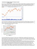
Figure 9. Continued
Foundations of Technical Analysis 1745
Table III
Summary statistics ~mean, standard deviation, skewness, and excess kurtosis! of raw and conditional one-day normalized returns of NYSE0
AMEX stocks from 1962 to 1996, in five-year subperiods, and in size quintiles. Conditional returns are defined as the daily return three days
following the conclusion of an occurrence of one of 10 technical indicators: head-and-shoulders ~HS!, inverted head-and-shoulders ~IHS!, broad-
ening top ~BTOP!, broadening bottom ~BBOT!, triangle top ~TTOP!, triangle bottom ~TBOT!, rectangle top ~RTOP!, rectangle bottom ~RBOT!,
double top ~DTOP!, and double bottom ~DBOT!. All returns have been normalized by subtraction of their means and division by their standard
deviations.
Moment Raw HS IHS BTOP BBOT TTOP TBOT RTOP RBOT DTOP DBOT
All Stocks, 1962 to 1996
Mean Ϫ0.000 Ϫ0.038 0.040 Ϫ0.005 Ϫ0.062 0.021 Ϫ0.009 0.009 0.014 0.017 Ϫ0.001
S.D. 1.000 0.867 0.937 1.035 0.979 0.955 0.959 0.865 0.883 0.910 0.999
Skew. 0.345 0.135 0.660 Ϫ1.151 0.090 0.137 0.643 Ϫ0.420 0.110 0.206 0.460
Kurt. 8.122 2.428 4.527 16.701 3.169 3.293 7.061 7.360 4.194 3.386 7.374
Smallest Quintile, 1962 to 1996
Mean Ϫ0.000 Ϫ0.014 0.036 Ϫ0.093 Ϫ0.188 0.036 Ϫ0.020 0.037 Ϫ0.093 0.043 Ϫ0.055
S.D. 1.000 0.854 1.002 0.940 0.850 0.937 1.157 0.833 0.986 0.950 0.962
Skew. 0.697 0.802 1.337 Ϫ1.771 Ϫ0.367 0.861 2.592 Ϫ0.187 0.445 0.511 0.002
Kurt. 10.873 3.870 7.143 6.701 0.575 4.185 12.532 1.793 4.384 2.581 3.989
2nd Quintile, 1962 to 1996
Mean Ϫ0.000 Ϫ0.069 0.144 0.061 Ϫ0.113 0.003 0.035 0.018 0.019 0.067 Ϫ0.011
S.D. 1.000 0.772 1.031 1.278 1.004 0.913 0.965 0.979 0.868 0.776 1.069
Skew. 0.392 0.223 1.128 Ϫ3.296 0.485 Ϫ0.529 0.166 Ϫ1.375 0.452 0.392 1.728
Kurt. 7.836 0.657 6.734 32.750 3.779 3.024 4.987 17.040 3.914 2.151 15.544
3rd Quintile, 1962 to 1996
Mean Ϫ0.000 Ϫ0.048 Ϫ0.043 Ϫ0.076 Ϫ0.056 0.036 0.012 0.075 0.028 Ϫ0.039 Ϫ0.034
S.D. 1.000 0.888 0.856 0.894 0.925 0.973 0.796 0.798 0.892 0.956 1.026
Skew. 0.246 Ϫ0.465 0.107 Ϫ0.023 0.233 0.538 0.166 0.678 Ϫ0.618 0.013 Ϫ0.242

Kurt. 7.466 3.239 1.612 1.024 0.611 2.995 0.586 3.010 4.769 4.517 3.663
4th Quintile, 1962 to 1996
Mean Ϫ0.000 Ϫ0.012 0.022 0.115 0.028 0.022 Ϫ0.014 Ϫ0.113 0.065 0.015 Ϫ0.006
S.D. 1.000 0.964 0.903 0.990 1.093 0.986 0.959 0.854 0.821 0.858 0.992
Skew. 0.222 0.055 0.592 0.458 0.537 Ϫ0.217 Ϫ0.456 Ϫ0.415 0.820 0.550 Ϫ0.062
Kurt. 6.452 1.444 1.745 1.251 2.168 4.237 8.324 4.311 3.632 1.719 4.691
Largest Quintile, 1962 to 1996
Mean Ϫ0.000 Ϫ0.038 0.054 Ϫ0.081 Ϫ0.042 0.010 Ϫ0.049 0.009 0.060 0.018 0.067
S.D. 1.000 0.843 0.927 0.997 0.951 0.964 0.965 0.850 0.820 0.971 0.941
Skew. 0.174 0.438 0.182 0.470 Ϫ1.099 0.089 0.357 Ϫ0.167 Ϫ0.140 0.011 0.511
Kurt. 7.992 2.621 3.465 3.275 6.603 2.107 2.509 0.816 3.179 3.498 5.035
1746 The Journal of Finance
All Stocks, 1962 to 1966
Mean Ϫ0.000 0.070 0.090 0.159 0.079 Ϫ0.033 Ϫ0.039 Ϫ0.041 0.019 Ϫ0.071 Ϫ0.100
S.D. 1.000 0.797 0.925 0.825 1.085 1.068 1.011 0.961 0.814 0.859 0.962
Skew. 0.563 0.159 0.462 0.363 1.151 Ϫ0.158 1.264 Ϫ1.337 Ϫ0.341 Ϫ0.427 Ϫ0.876
Kurt. 9.161 0.612 1.728 0.657 5.063 2.674 4.826 17.161 1.400 3.416 5.622
All Stocks, 1967 to 1971
Mean Ϫ0.000 Ϫ0.044 0.079 Ϫ0.035 Ϫ0.056 0.025 0.057 Ϫ0.101 0.110 0.093 0.079
S.D. 1.000 0.809 0.944 0.793 0.850 0.885 0.886 0.831 0.863 1.083 0.835
Skew. 0.342 0.754 0.666 0.304 0.085 0.650 0.697 Ϫ1.393 0.395 1.360 0.701
Kurt. 5.810 3.684 2.725 0.706 0.141 3.099 1.659 8.596 3.254 4.487 1.853
All Stocks, 1972 to 1976
Mean Ϫ0.000 Ϫ0.035 0.043 0.101 Ϫ0.138 Ϫ0.045 Ϫ0.010 Ϫ0.025 Ϫ0.003 Ϫ0.051 Ϫ0.108
S.D. 1.000 1.015 0.810 0.985 0.918 0.945 0.922 0.870 0.754 0.914 0.903
Skew. 0.316 Ϫ0.334 0.717 Ϫ0.699 0.272 Ϫ1.014 0.676 0.234 0.199 0.056 Ϫ0.366
Kurt. 6.520 2.286 1.565 6.562 1.453 5.261 4.912 3.627 2.337 3.520 5.047
All Stocks, 1977 to 1981
Mean Ϫ0.000 Ϫ0.138 Ϫ0.040 0.076 Ϫ0.114 0.135 Ϫ0.050 Ϫ0.004 0.026 0.042 0.178
S.D. 1.000 0.786 0.863 1.015 0.989 1.041 1.011 0.755 0.956 0.827 1.095

Skew. 0.466 Ϫ0.304 0.052 1.599 Ϫ0.033 0.776 0.110 Ϫ0.084 0.534 0.761 2.214
Kurt. 6.419 1.132 1.048 4.961 Ϫ0.125 2.964 0.989 1.870 2.184 2.369 15.290
All Stocks, 1982 to 1986
Mean Ϫ0.000 Ϫ0.099 Ϫ0.007 0.011 0.095 Ϫ0.114 Ϫ0.067 0.050 0.005 0.011 Ϫ0.013
S.D. 1.000 0.883 1.002 1.109 0.956 0.924 0.801 0.826 0.934 0.850 1.026
Skew. 0.460 0.464 0.441 0.372 Ϫ0.165 0.473 Ϫ1.249 0.231 0.467 0.528 0.867
Kurt. 6.799 2.280 6.128 2.566 2.735 3.208 5.278 1.108 4.234 1.515 7.400
All Stocks, 1987 to 1991
Mean Ϫ0.000 Ϫ0.037 0.033 Ϫ0.091 Ϫ0.040 0.053 0.003 0.040 Ϫ0.020 Ϫ0.022 Ϫ0.017
S.D. 1.000 0.848 0.895 0.955 0.818 0.857 0.981 0.894 0.833 0.873 1.052
Skew. Ϫ0.018 Ϫ0.526 0.272 0.108 0.231 0.165 Ϫ1.216 0.293 0.124 Ϫ1.184 Ϫ0.368
Kurt. 13.478 3.835 4.395 2.247 1.469 4.422 9.586 1.646 3.973 4.808 4.297
All Stocks, 1992 to 1996
Mean Ϫ0.000 Ϫ0.014 0.069 Ϫ0.231 Ϫ0.272 0.122 0.041 0.082 0.011 0.102 Ϫ0.016
S.D. 1.000 0.935 1.021 1.406 1.187 0.953 1.078 0.814 0.996 0.960 1.035
Skew. 0.308 0.545 1.305 Ϫ3.988 Ϫ0.502 Ϫ0.190 2.460 Ϫ0.167 Ϫ0.129 Ϫ0.091 0.379
Kurt. 8.683 2.249 6.684 27.022 3.947 1.235 12.883 0.506 6.399 1.507 3.358
Foundations of Technical Analysis 1747
Table IV
Summary statistics ~mean, standard deviation, skewness, and excess kurtosis! of raw and conditional one-day normalized returns of Nasdaq
stocks from 1962 to 1996, in five-year subperiods, and in size quintiles. Conditional returns are defined as the daily return three days following
the conclusion of an occurrence of one of 10 technical indicators: head-and-shoulders ~HS!, inverted head-and-shoulders ~IHS!, broadening top
~BTOP!, broadening bottom ~BBOT!, triangle top ~TTOP!, triangle bottom ~TBOT!, rectangle top ~RTOP!, rectangle bottom ~RBOT!, double top
~DTOP!, and double bottom ~DBOT!. All returns have been normalized by subtraction of their means and division by their standard deviations.
Moment Raw HS IHS BTOP BBOT TTOP TBOT RTOP RBOT DTOP DBOT
All Stocks, 1962 to 1996
Mean 0.000 Ϫ0.016 0.042 Ϫ0.009 0.009 Ϫ0.020 0.017 0.052 0.043 0.003 Ϫ0.035
S.D. 1.000 0.907 0.994 0.960 0.995 0.984 0.932 0.948 0.929 0.933 0.880
Skew. 0.608 Ϫ0.017 1.290 0.397 0.586 0.895 0.716 0.710 0.755 0.405 Ϫ0.104
Kurt. 12.728 3.039 8.774 3.246 2.783 6.692 3.844 5.173 4.368 4.150 2.052

Smallest Quintile, 1962 to 1996
Mean Ϫ0.000 0.018 Ϫ0.032 0.087 Ϫ0.153 0.059 0.108 0.136 0.013 0.040 0.043
S.D. 1.000 0.845 1.319 0.874 0.894 1.113 1.044 1.187 0.982 0.773 0.906
Skew. 0.754 0.325 1.756 Ϫ0.239 Ϫ0.109 2.727 2.300 1.741 0.199 0.126 Ϫ0.368
Kurt. 15.859 1.096 4.221 1.490 0.571 14.270 10.594 8.670 1.918 0.127 0.730
2nd Quintile, 1962 to 1996
Mean Ϫ0.000 Ϫ0.064 0.076 Ϫ0.109 Ϫ0.093 Ϫ0.085 Ϫ0.038 Ϫ0.066 Ϫ0.015 0.039 Ϫ0.034
S.D. 1.000 0.848 0.991 1.106 1.026 0.805 0.997 0.898 0.897 1.119 0.821
Skew. 0.844 0.406 1.892 Ϫ0.122 0.635 0.036 0.455 Ϫ0.579 0.416 1.196 0.190
Kurt. 16.738 2.127 11.561 2.496 3.458 0.689 1.332 2.699 3.871 3.910 0.777
3rd Quintile, 1962 to 1996
Mean Ϫ0.000 0.033 0.028 0.078 0.210 Ϫ0.030 0.068 0.117 0.210 Ϫ0.109 Ϫ0.075
S.D. 1.000 0.933 0.906 0.931 0.971 0.825 1.002 0.992 0.970 0.997 0.973
Skew. 0.698 0.223 0.529 0.656 0.326 0.539 0.442 0.885 0.820 Ϫ0.163 0.123
Kurt. 12.161 1.520 1.526 1.003 0.430 1.673 1.038 2.908 4.915 5.266 2.573
4th Quintile, 1962 to 1996
Mean 0.000 Ϫ0.079 0.037 Ϫ0.006 Ϫ0.044 Ϫ0.080 0.007 0.084 0.044 0.038 Ϫ0.048
S.D. 1.000 0.911 0.957 0.992 0.975 1.076 0.824 0.890 0.851 0.857 0.819
Skew. 0.655 Ϫ0.456 2.671 Ϫ0.174 0.385 0.554 0.717 0.290 1.034 0.154 Ϫ0.149
Kurt. 11.043 2.525 19.593 2.163 1.601 7.723 3.930 1.555 2.982 2.807 2.139
Largest Quintile, 1962 to 1996
Mean 0.000 0.026 0.058 Ϫ0.070 0.031 0.052 Ϫ0.013 0.001 Ϫ0.024 0.032 Ϫ0.018
S.D. 1.000 0.952 1.002 0.895 1.060 1.076 0.871 0.794 0.958 0.844 0.877
Skew. 0.100 Ϫ0.266 Ϫ0.144 1.699 1.225 0.409 0.025 0.105 1.300 0.315 Ϫ0.363
Kurt. 7.976 5.807 4.367 8.371 5.778 1.970 2.696 1.336 7.503 2.091 2.241
1748 The Journal of Finance
All Stocks, 1962 to 1966
Mean Ϫ0.000 0.116 0.041 0.099 0.090 0.028 Ϫ0.066 0.100 0.010 0.096 0.027
S.D. 1.000 0.912 0.949 0.989 1.039 1.015 0.839 0.925 0.873 1.039 0.840
Skew. 0.575 0.711 1.794 0.252 1.258 1.601 0.247 2.016 1.021 0.533 Ϫ0.351

Kurt. 6.555 1.538 9.115 2.560 6.445 7.974 1.324 13.653 5.603 6.277 2.243
All Stocks, 1967 to 1971
Mean Ϫ0.000 Ϫ0.127 0.114 0.121 0.016 0.045 0.077 0.154 0.136 Ϫ0.000 0.006
S.D. 1.000 0.864 0.805 0.995 1.013 0.976 0.955 1.016 1.118 0.882 0.930
Skew. 0.734 Ϫ0.097 1.080 0.574 0.843 1.607 0.545 0.810 1.925 0.465 0.431
Kurt. 5.194 1.060 2.509 0.380 2.928 10.129 1.908 1.712 5.815 1.585 2.476
All Stocks, 1972 to 1976
Mean 0.000 0.014 0.089 Ϫ0.403 Ϫ0.034 Ϫ0.132 Ϫ0.422 Ϫ0.076 0.108 Ϫ0.004 Ϫ0.163
S.D. 1.000 0.575 0.908 0.569 0.803 0.618 0.830 0.886 0.910 0.924 0.564
Skew. 0.466 Ϫ0.281 0.973 Ϫ1.176 0.046 Ϫ0.064 Ϫ1.503 Ϫ2.728 2.047 Ϫ0.551 Ϫ0.791
Kurt. 17.228 2.194 1.828 0.077 0.587 Ϫ0.444 2.137 13.320 9.510 1.434 2.010
All Stocks, 1977 to 1981
Mean Ϫ0.000 0.025 Ϫ0.212 Ϫ0.112 Ϫ0.056 Ϫ0.110 0.086 0.055 0.177 0.081 0.040
S.D. 1.000 0.769 1.025 1.091 0.838 0.683 0.834 1.036 1.047 0.986 0.880
Skew. 1.092 0.230 Ϫ1.516 Ϫ0.731 0.368 0.430 0.249 2.391 2.571 1.520 Ϫ0.291
Kurt. 20.043 1.618 4.397 3.766 0.460 0.962 4.722 9.137 10.961 7.127 3.682
All Stocks, 1982 to 1986
Mean 0.000 Ϫ0.147 0.204 Ϫ0.137 Ϫ0.001 Ϫ0.053 Ϫ0.022 Ϫ0.028 0.116 Ϫ0.224 Ϫ0.052
S.D. 1.000 1.073 1.442 0.804 1.040 0.982 1.158 0.910 0.830 0.868 1.082
Skew. 1.267 Ϫ1.400 2.192 0.001 0.048 1.370 1.690 Ϫ0.120 0.048 0.001 Ϫ0.091
Kurt. 21.789 4.899 10.530 0.863 0.732 8.460 7.086 0.780 0.444 1.174 0.818
All Stocks, 1987 to 1991
Mean 0.000 0.012 0.120 Ϫ0.080 Ϫ0.031 Ϫ0.052 0.038 0.098 0.049 Ϫ0.048 Ϫ0.122
S.D. 1.000 0.907 1.136 0.925 0.826 1.007 0.878 0.936 1.000 0.772 0.860
Skew. 0.104 Ϫ0.326 0.976 Ϫ0.342 0.234 Ϫ0.248 1.002 0.233 0.023 Ϫ0.105 Ϫ0.375
Kurt. 12.688 3.922 5.183 1.839 0.734 2.796 2.768 1.038 2.350 0.313 2.598
All Stocks, 1992 to 1996
Mean 0.000 Ϫ0.119 Ϫ0.058 Ϫ0.033 Ϫ0.013 Ϫ0.078 0.086 Ϫ0.006 Ϫ0.011 0.003 Ϫ0.105
S.D. 1.000 0.926 0.854 0.964 1.106 1.093 0.901 0.973 0.879 0.932 0.875
Skew. Ϫ0.036 0.079 Ϫ0.015 1.399 0.158 Ϫ0.127 0.150 0.283 0.236 0.039 Ϫ0.097

Kurt. 5.377 2.818 Ϫ0.059 7.584 0.626 2.019 1.040 1.266 1.445 1.583 0.205
Foundations of Technical Analysis 1749
Table V
Goodness-of-fit diagnostics for the conditional one-day normalized returns, conditional on 10 technical indicators, for a sample of 350 NYSE0AMEX
stocks from 1962 to 1996 ~10 stocks per size-quintile with at least 80% nonmissing prices are randomly chosen in each five-year subperiod, yielding
50 stocks per subperiod over seven subperiods!. For each pattern, the percentage of conditional returns that falls within each of the 10 unconditional-
return deciles is tabulated. If conditioning on the pattern provides no information, the expected percentage falling in each decile is 10%. Asymptotic
z-statistics for this null hypothesis are reported in parentheses, and the x
2
goodness-of-fitness test statistic Q is reported in the last column with
the p-value in parentheses below the statistic. The 10 technical indicators are as follows: head-and-shoulders ~HS!, inverted head-and-shoulders
~IHS!, broadening top ~BTOP!, broadening bottom ~BBOT!, triangle top ~TTOP!, triangle bottom ~TBOT!, rectangle top ~RTOP!, rectangle bottom
~RBOT!, double top ~DTOP!, and double bottom ~DBOT!.
Decile:
Pattern 1 2 3 4 5678910
Q
~p-Value!
HS 8.9 10.4 11.2 11.7 12.2 7.9 9.2 10.4 10.8 7.1 39.31
~Ϫ1.49!~0.56!~1.49!~2.16!~2.73!~Ϫ3.05!~Ϫ1.04!~0.48!~1.04!~Ϫ4.46!~0.000!
IHS 8.6 9.7 9.4 11.2 13.7 7.7 9.1 11.1 9.6 10.0 40.95
~Ϫ2.05!~Ϫ0.36!~Ϫ0.88!~1.60!~4.34!~Ϫ3.44!~Ϫ1.32!~1.38!~Ϫ0.62!~Ϫ0.03!~0.000!
BTOP 9.4 10.6 10.6 11.9 8.7 6.6 9.2 13.7 9.2 10.1 23.40
~Ϫ0.57!~0.54!~0.54!~1.55!~Ϫ1.25!~Ϫ3.66!~Ϫ0.71!~2.87!~Ϫ0.71!~0.06!~0.005!
BBOT 11.5 9.9 13.0 11.1 7.8 9.2 8.3 9.0 10.7 9.6 16.87
~1.28!~Ϫ0.10!~2.42!~0.95!~Ϫ2.30!~Ϫ0.73!~Ϫ1.70!~Ϫ1.00!~0.62!~Ϫ0.35!~0.051!
TTOP 7.8 10.4 10.9 11.3 9.0 9.9 10.0 10.7 10.5 9.7 12.03
~Ϫ2.94!~0.42!~1.03!~1.46!~Ϫ1.30!~Ϫ0.13!~Ϫ0.04!~0.77!~0.60!~Ϫ0.41!~0.212!
TBOT 8.9 10.6 10.9 12.2 9.2 8.7 9.3 11.6 8.7 9.8 17.12
~Ϫ1.35!~0.72!~0.99!~2.36!~Ϫ0.93!~Ϫ1.57!~Ϫ0.83!~1.69!~Ϫ1.57!~Ϫ0.22!~0.047!
RTOP 8.4 9.9 9.2 10.5 12.5 10.1 10.0 10.0 11.4 8.1 22.72

~Ϫ2.27!~Ϫ0.10!~Ϫ1.10!~0.58!~2.89!~0.16!~Ϫ0.02!~Ϫ0.02!~1.70!~Ϫ2.69!~0.007!
RBOT 8.6 9.6 7.8 10.5 12.9 10.8 11.6 9.3 10.3 8.7 33.94
~Ϫ2.01!~Ϫ0.56!~Ϫ3.30!~0.60!~3.45!~1.07!~1.98!~Ϫ0.99!~0.44!~Ϫ1.91!~0.000!
DTOP 8.2 10.9 9.6 12.4 11.8 7.5 8.2 11.3 10.3 9.7 50.97
~Ϫ2.92!~1.36!~Ϫ0.64!~3.29!~2.61!~Ϫ4.39!~Ϫ2.92!~1.83!~0.46!~Ϫ0.41!~0.000!
DBOT 9.7 9.9 10.0 10.9 11.4 8.5 9.2 10.0 10.7 9.8 12.92
~Ϫ0.48!~Ϫ0.18!~Ϫ0.04!~1.37!~1.97!~Ϫ2.40!~Ϫ1.33!~0.04!~0.96!~Ϫ0.33!~0.166!
1750 The Journal of Finance
Table VI
Goodness-of-fit diagnostics for the conditional one-day normalized returns, conditional on 10 technical indicators, for a sample of 350 Nasdaq stocks
from 1962 to 1996 ~10 stocks per size-quintile with at least 80% nonmissing prices are randomly chosen in each five-year subperiod, yielding 50
stocks per subperiod over seven subperiods!. For each pattern, the percentage of conditional returns that falls within each of the 10 unconditional-
return deciles is tabulated. If conditioning on the pattern provides no information, the expected percentage falling in each decile is 10%. Asymptotic
z-statistics for this null hypothesis are reported in parentheses, and the x
2
goodness-of-fitness test statistic Q is reported in the last column with
the p-value in parentheses below the statistic. The 10 technical indicators are as follows: head-and-shoulders ~HS!, inverted head-and-shoulders
~IHS!, broadening top ~BTOP!, broadening bottom ~BBOT!, triangle top ~TTOP!, triangle bottom ~TBOT!, rectangle top ~RTOP!, rectangle bottom
~RBOT!, double top ~DTOP!, and double bottom ~DBOT!.
Decile:
Pattern 1 2 345678910
Q
~p-Value!
HS 10.8 10.8 13.7 8.6 8.5 6.0 6.0 12.5 13.5 9.7 64.41
~0.76!~0.76!~3.27!~Ϫ1.52!~Ϫ1.65!~Ϫ5.13!~Ϫ5.13!~2.30!~3.10!~Ϫ0.32!~0.000!
IHS 9.4 14.1 12.5 8.0 7.7 4.8 6.4 13.5 12.5 11.3 75.84
~Ϫ0.56!~3.35!~2.15!~Ϫ2.16!~Ϫ2.45!~Ϫ7.01!~Ϫ4.26!~2.90!~2.15!~1.14!~0.000!
BTOP 11.6 12.3 12.8 7.7 8.2 6.8 4.3 13.3 12.1 10.9 34.12
~1.01!~1.44!~1.71!~Ϫ1.73!~Ϫ1.32!~Ϫ2.62!~Ϫ5.64!~1.97!~1.30!~0.57!~0.000!
BBOT 11.4 11.4 14.8 5.9 6.7 9.6 5.7 11.4 9.8 13.2 43.26

~1.00!~1.00!~3.03!~Ϫ3.91!~Ϫ2.98!~Ϫ0.27!~Ϫ4.17!~1.00!~Ϫ0.12!~2.12!~0.000!
TTOP 10.7 12.1 16.2 6.2 7.9 8.7 4.0 12.5 11.4 10.2 92.09
~0.67!~1.89!~4.93!~Ϫ4.54!~Ϫ2.29!~Ϫ1.34!~Ϫ8.93!~2.18!~1.29!~0.23!~0.000!
TBOT 9.9 11.3 15.6 7.9 7.7 5.7 5.3 14.6 12.0 10.0 85.26
~Ϫ0.11!~1.14!~4.33!~Ϫ2.24!~Ϫ2.39!~Ϫ5.20!~Ϫ5.85!~3.64!~1.76!~0.01!~0.000!
RTOP 11.2 10.8 8.8 8.3 10.2 7.1 7.7 9.3 15.3 11.3 57.08
~1.28!~0.92!~Ϫ1.40!~Ϫ2.09!~0.25!~Ϫ3.87!~Ϫ2.95!~Ϫ0.75!~4.92!~1.37!~0.000!
RBOT 8.9 12.3 8.9 8.9 11.6 8.9 7.0 9.5 13.6 10.3 45.79
~Ϫ1.35!~2.52!~Ϫ1.35!~Ϫ1.45!~1.81!~Ϫ1.35!~Ϫ4.19!~Ϫ0.66!~3.85!~0.36!~0.000!
DTOP 11.0 12.6 11.7 9.0 9.2 5.5 5.8 11.6 12.3 11.3 71.29
~1.12!~2.71!~1.81!~Ϫ1.18!~Ϫ0.98!~Ϫ6.76!~Ϫ6.26!~1.73!~2.39!~1.47!~0.000!
DBOT 10.9 11.5 13.1 8.0 8.1 7.1 7.6 11.5 12.8 9.3 51.23
~0.98!~1.60!~3.09!~Ϫ2.47!~Ϫ2.35!~Ϫ3.75!~Ϫ3.09!~1.60!~2.85!~Ϫ0.78!~0.000!
Foundations of Technical Analysis 1751
in the Nasdaq sample, with p-values that are zero to three significant digits
and test statistics Q that range from 34.12 to 92.09. In contrast, the test
statistics in Table V range from 12.03 to 50.97.
One possible explanation for the difference between the NYSE0AMEX and
Nasdaq samples is a difference in the power of the test because of different
sample sizes. If the NYSE0AMEX sample contained fewer conditional re-
turns, that is, fewer patterns, the corresponding test statistics might be sub-
ject to greater sampling variation and lower power. However, this explanation
can be ruled out from the frequency counts of Tables I and II—the number
of patterns in the NYSE0AMEX sample is considerably larger than those of
the Nasdaq sample for all 10 patterns. Tables V and VI seem to suggest
important differences in the informativeness of technical indicators for NYSE0
AMEX and Nasdaq stocks.
Table VII and VIII report the results of the Kolmogorov–Smirnov test ~equa-
tion ~19!! of the equality of the conditional and unconditional return distri-
butions for NYSE0AMEX ~Table VII! and Nasdaq ~Table VIII! stocks,

respectively, from 1962 to 1996, in five-year subperiods and in market-
capitalization quintiles. Recall that conditional returns are defined as the
one-day return starting three days following the conclusion of an occurrence
of a pattern. The p-values are with respect to the asymptotic distribution of
the Kolmogorov–Smirnov test statistic given in equation ~20!. Table VII shows
that for NYSE0AMEX stocks, five of the 10 patterns—HS, BBOT, RTOP,
RBOT, and DTOP—yield statistically significant test statistics, with p-values
ranging from 0.000 for RBOT to 0.021 for DTOP patterns. However, for the
other five patterns, the p-values range from 0.104 for IHS to 0.393 for TTOP,
which implies an inability to distinguish between the conditional and un-
conditional distributions of normalized returns.
When we also condition on declining volume trend, the statistical signif-
icance declines for most patterns, but the statistical significance of TBOT
patterns increases. In contrast, conditioning on increasing volume trend yields
an increase in the statistical significance of BTOP patterns. This difference
may suggest an important role for volume trend in TBOT and BTOP pat-
terns. The difference between the increasing and decreasing volume-trend
conditional distributions is statistically insignificant for almost all the pat-
terns ~the sole exception is the TBOT pattern!. This drop in statistical sig-
nificance may be due to a lack of power of the Kolmogorov–Smirnov test
given the relatively small sample sizes of these conditional returns ~see Table I
for frequency counts!.
Table VIII reports corresponding results for the Nasdaq sample, and as in
Table VI, in contrast to the NYSE0AMEX results, here all the patterns are
statistically significant at the 5 percent level. This is especially significant
because the the Nasdaq sample exhibits far fewer patterns than the NYSE0
AMEX sample ~see Tables I and II!, and hence the Kolmogorov–Smirnov test
is likely to have lower power in this case.
As with the NYSE0AMEX sample, volume trend seems to provide little
incremental information for the Nasdaq sample except in one case: increas-

ing volume and BTOP. And except for the TTOP pattern, the Kolmogorov–
1752 The Journal of Finance
Smirnov test still cannot distinguish between the decreasing and in-
creasing volume-trend conditional distributions, as the last pair of rows of
Table VIII’s first panel indicates.
IV. Monte Carlo Analysis
Tables IX and X contain bootstrap percentiles for the Kolmogorov–
Smirnov test of the equality of conditional and unconditional one-day return
distributions for NYSE0AMEX and Nasdaq stocks, respectively, from 1962 to
1996, for five-year subperiods, and for market-capitalization quintiles, un-
der the null hypothesis of equality. For each of the two sets of market data,
two sample sizes, m
1
and m
2
, have been chosen to span the range of fre-
quency counts of patterns reported in Tables I and II. For each sample size
m
i
, we resample one-day normalized returns ~with replacement! to obtain a
bootstrap sample of m
i
observations, compute the Kolmogorov–Smirnov test
statistic ~against the entire sample of one-day normalized returns!, and re-
peat this procedure 1,000 times. The percentiles of the asymptotic distribu-
tion are also reported for comparison in the column labeled “⌬”.
Tables IX and X show that for a broad range of sample sizes and across
size quintiles, subperiod, and exchanges, the bootstrap distribution of the
Kolmogorov–Smirnov statistic is well approximated by its asymptotic distri-
bution, equation ~20!.

V. Conclusion
In this paper, we have proposed a new approach to evaluating the efficacy
of technical analysis. Based on smoothing techniques such as nonparametric
kernel regression, our approach incorporates the essence of technical analy-
sis: to identify regularities in the time series of prices by extracting nonlin-
ear patterns from noisy data. Although human judgment is still superior to
most computational algorithms in the area of visual pattern recognition,
recent advances in statistical learning theory have had successful applica-
tions in fingerprint identification, handwriting analysis, and face recogni-
tion. Technical analysis may well be the next frontier for such methods.
We find that certain technical patterns, when applied to many stocks over
many time periods, do provide incremental information, especially for Nas-
daq stocks. Although this does not necessarily imply that technical analysis
can be used to generate “excess” trading profits, it does raise the possibility
that technical analysis can add value to the investment process.
Moreover, our methods suggest that technical analysis can be improved by
using automated algorithms such as ours and that traditional patterns such
as head-and-shoulders and rectangles, although sometimes effective, need
not be optimal. In particular, it may be possible to determine “optimal pat-
terns” for detecting certain types of phenomena in financial time series, for
example, an optimal shape for detecting stochastic volatility or changes in
regime. Moreover, patterns that are optimal for detecting statistical anom-
alies need not be optimal for trading profits, and vice versa. Such consider-
Foundations of Technical Analysis 1753
Table VII
Kolmogorov–Smirnov test of the equality of conditional and unconditional one-day return distributions for NYSE0AMEX stocks from 1962 to
1996, in five-year subperiods, and in size quintiles. Conditional returns are defined as the daily return three days following the conclusion of an
occurrence of one of 10 technical indicators: head-and-shoulders ~HS!, inverted head-and-shoulders ~IHS!, broadening top ~BTOP!, broadening
bottom ~BBOT!, triangle top ~TTOP!, triangle bottom ~TBOT!, rectangle top ~RTOP!, rectangle bottom ~RBOT!, double top ~DTOP!, and double
bottom ~DBOT!. All returns have been normalized by subtraction of their means and division by their standard deviations. p-values are with

respect to the asymptotic distribution of the Kolmogorov–Smirnov test statistic. The symbols “t~
'
!” and “t~
;
!” indicate that the conditional
distribution is also conditioned on decreasing and increasing volume trend, respectively.
Statistic HS IHS BTOP BBOT TTOP TBOT RTOP RBOT DTOP DBOT
All Stocks, 1962 to 1996
g 1.89 1.22 1.15 1.76 0.90 1.09 1.84 2.45 1.51 1.06
p-value 0.002 0.104 0.139 0.004 0.393 0.185 0.002 0.000 0.021 0.215
gt~
'
! 1.49 0.95 0.44 0.62 0.73 1.33 1.37 1.77 0.96 0.78
p-value 0.024 0.327 0.989 0.839 0.657 0.059 0.047 0.004 0.319 0.579
gt~
;
! 0.72 1.05 1.33 1.59 0.92 1.29 1.13 1.24 0.74 0.84
p-value 0.671 0.220 0.059 0.013 0.368 0.073 0.156 0.090 0.638 0.481
g Diff. 0.88 0.54 0.59 0.94 0.75 1.37 0.79 1.20 0.82 0.71
p-value 0.418 0.935 0.879 0.342 0.628 0.046 0.557 0.111 0.512 0.698
Smallest Quintile, 1962 to 1996
g 0.59 1.19 0.72 1.20 0.98 1.43 1.09 1.19 0.84 0.78
p-value 0.872 0.116 0.679 0.114 0.290 0.033 0.188 0.120 0.485 0.583
gt~
'
! 0.67 0.80 1.16 0.69 1.00 1.46 1.31 0.94 1.12 0.73
p-value 0.765 0.540 0.136 0.723 0.271 0.029 0.065 0.339 0.165 0.663
gt~
;
! 0.43 0.95 0.67 1.03 0.47 0.88 0.51 0.93 0.94 0.58

p-value 0.994 0.325 0.756 0.236 0.981 0.423 0.959 0.356 0.342 0.892
g Diff. 0.52 0.48 1.14 0.68 0.48 0.98 0.98 0.79 1.16 0.62
p-value 0.951 0.974 0.151 0.741 0.976 0.291 0.294 0.552 0.133 0.840
2nd Quintile, 1962 to 1996
g 1.82 1.63 0.93 0.92 0.82 0.84 0.88 1.29 1.46 0.84
p