A HEAT TRANSFER TEXTBOOK - THIRD EDITION Episode 1 Part 8 pps

Figure 4.6 Some of the many varieties of finned tubes.
164
§4.5 Fin design 165
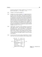
Figure 4.7 The Stegosaurus with what
might have been cooling fins (etching by
Daniel Rosner).
ing, condensing, or other natural convection situations, and will not be
strictly accurate even in forced convection.
The tip may or may not exchange heat with the surroundings through
a heat transfer coefficient,
h
L
, which would generally differ from h. The
length of the fin is L, its uniform cross-sectional area is A, and its cir-
cumferential perimeter is P.
The characteristic dimension of the fin in the transverse direction
(normal to the x-axis) is taken to be A/P. Thus, for a circular cylindrical
fin, A/P = π(radius)
2
/(2π radius) = (radius/2). We define a Biot num-
ber for conduction in the transverse direction, based on this dimension,
and require that it be small:
Bi
fin
=
h(A/P)
k
 1 (4.27)
This condition means that the transverse variation of T at any axial po-
sition, x, is much less than (T
surface

−T
∞
). Thus, T  T(x only) and the
166 Analysis of heat conduction and some steady one-dimensional problems §4.5
Figure 4.8 The analysis of a one-dimensional fin.
heat flow can be treated as one-dimensional.
An energy balance on the thin slice of the fin shown in Fig. 4.8 gives
−kA
dT
dx




x+δx
+kA
dT
dx




x
+h(Pδx)(T −T
∞
)
x
= 0 (4.28)
but
dT /dx|

x+δx
− dT/dx|
x
δx
→
d
2
T
dx
2
=
d
2
(T −T
∞
)
dx
2
(4.29)
so
d
2
(T −T
∞
)
dx
2
=
hP
kA

(T −T
∞
) (4.30)
§4.5 Fin design 167
The b.c.’s for this equation are
(T −T
∞
)
x=0
= T
0
−T
∞
−kA
d(T −T
∞
)
dx




x=L
= h
L
A(T −T
∞
)
x=L
(4.31a)

Alternatively, if the tip is insulated, or if we can guess that
h
L
is small
enough to be unimportant, the b.c.’s are
(T −T
∞
)
x=0
= T
0
−T
∞
and
d(T −T
∞
)
dx




x=L
= 0 (4.31b)
Before we solve this problem, it will pay to do a dimensional analysis of
it. The dimensional functional equation is
T −T
∞
= fn


(
T
0
−T
∞
)
,x,L,kA,hP, h
L
A

(4.32)
Notice that we have written kA,
hP, and h
L
A as single variables. The
reason for doing so is subtle but important. Setting h(A/P)/k  1,
erases any geometric detail of the cross section from the problem. The
only place where P and A enter the problem is as product of k,
h, orh
L
.
If they showed up elsewhere, they would have to do so in a physically
incorrect way. Thus, we have just seven variables in W, K, and m. This
gives four pi-groups if the tip is uninsulated:
T −T
∞
T
0
−T
∞

= fn







x
L
,

hP
kA
L
2
,
h
L
AL
kA

 
=h
L
L

k








or if we rename the groups,
Θ = fn
(
ξ,mL,Bi
axial
)
(4.33a)
where we call

hPL
2
/kA ≡ mL because that terminology is common in
the literature on fins.
If the tip of the fin is insulated,
h
L
will not appear in eqn. (4.32). There
is one less variable but the same number of dimensions; hence, there will
be only three pi-groups. The one that is removed is Bi
axial
, which involves
h
L
. Thus, for the insulated fin,
Θ = fn(ξ, mL) (4.33b)

168 Analysis of heat conduction and some steady one-dimensional problems §4.5
We put eqn. (4.30) in these terms by multiplying it by L
2
/(T
0
−T
∞
). The
result is
d
2
Θ
dξ
2
= (mL)
2
Θ (4.34)
This equation is satisfied by Θ = Ce
±(mL)ξ
. The sum of these two solu-
tions forms the general solution of eqn. (4.34):
Θ = C
1
e
mLξ
+C
2
e
−mLξ
(4.35)

Temperature distribution in a one-dimensional fin with the tip insu-
lated The b.c.’s [eqn. (4.31b)] can be written as
Θ
ξ=0
= 1 and
dΘ
dξ





ξ=1
= 0 (4.36)
Substituting eqn. (4.35) into both eqns. (4.36), we get
C
1
+C
2
= 1 and C
1
e
mL
−C
2
e
−mL
= 0 (4.37)
Mathematical Digression 4.1
To put the solution of eqn. (4.37) for C

1
and C
2
in the simplest form,
we need to recall a few properties of hyperbolic functions. The four basic
functions that we need are defined as
sinh x ≡
e
x
−e
−x
2
cosh x ≡
e
x
+e
−x
2
tanh x ≡
sinh x
cosh x
=
e
x
−e
−x
e
x
+e
−x

coth x ≡
e
x
+e
−x
e
x
−e
−x
(4.38)
where x is the independent variable. Additional functions are defined
by analogy to the trigonometric counterparts. The differential relations
§4.5 Fin design 169
can be written out formally, and they also resemble their trigonometric
counterparts.
d
dx
sinh x =
1
2

e
x
−(−e
−x
)

= coshx
d
dx

cosh x =
1
2

e
x
+(−e
−x
)

= sinh x
(4.39)
These are analogous to the familiar results, d sin x/dx = cos x and
d cos x/dx =−sin x, but without the latter minus sign.
The solution of eqns. (4.37) is then
C
1
=
e
−mL
2 cosh mL
and C
2
= 1 −
e
−mL
2 cosh mL
(4.40)
Therefore, eqn. (4.35) becomes
Θ =

e
−mL(1−ξ)
+(2 cosh mL)e
−mLξ
−e
−mL(1+ξ)
2 cosh mL
which simplifies to
Θ =
cosh mL(1 − ξ)
cosh mL
(4.41)
for a one-dimensional fin with its tip insulated.
One of the most important design variables for a fin is the rate at
which it removes (or delivers) heat the wall. To calculate this, we write
Fourier’s law for the heat flow into the base of the fin:
6
Q =−kA
d(T −T
∞
)
dx




x=0
(4.42)
We multiply eqn. (4.42)byL/kA(T
0

− T
∞
) and obtain, after substituting
eqn. (4.41) on the right-hand side,
QL
kA(T
0
−T
∞
)
= mL
sinh mL
cosh mL
= mL tanh mL (4.43)
6
We could also integrate h(T − T
∞
) over the outside area of the fin to get Q. The
answer would be the same, but the calculation would be a little more complicated.
170 Analysis of heat conduction and some steady one-dimensional problems §4.5
Figure 4.9 The temperature distribution, tip temperature, and
heat flux in a straight one-dimensional fin with the tip insulated.
which can be written
Q

kAhP(T
0
−T
∞
)

= tanh mL (4.44)
Figure 4.9 includes two graphs showing the behavior of one-dimen-
sional fin with an insulated tip. The top graph shows how the heat re-
moval increases with mL to a virtual maximum at mL  3. This means
that no such fin should have a length in excess of 2/m or 3/m if it is be-
ing used to cool (or heat) a wall. Additional length would simply increase
the cost without doing any good.
Also shown in the top graph is the temperature of the tip of such a
fin. Setting ξ = 1 in eqn. (4.41), we discover that
Θ
tip
=
1
cosh mL
(4.45)
§4.5 Fin design 171
This dimensionless temperature drops to about 0.014 at the tip when mL
reaches 5. This means that the end is 0.014(T
0
− T
∞
) K above T
∞
at the
end. Thus, if the fin is actually functioning as a holder for a thermometer
or a thermocouple that is intended to read T
∞
, the reading will be in error
if mL is not significantly greater than five.
The lower graph in Fig. 4.9 hows how the temperature is distributed

in insulated-tip fins for various values of mL.
Experiment 4.1
Clamp a 20 cm or so length of copper rod by one end in a horizontal
position. Put a candle flame very near the other end and let the arrange-
ment come to a steady state. Run your finger along the rod. How does
what you feel correspond to Fig. 4.9? (The diameter for the rod should
not exceed about 3 mm. A larger rod of metal with a lower conductivity
will also work.)
Exact temperature distribution in a fin with an uninsulated tip. The
approximation of an insulated tip may be avoided using the b.c’s given
in eqn. (4.31a), which take the following dimensionless form:
Θ
ξ=0
= 1 and −
dΘ
dξ





ξ=1
= Bi
ax
Θ
ξ=1
(4.46)
Substitution of the general solution, eqn. (4.35), in these b.c.’s yields
C
1

+C
2
= 1
−mL(C
1
e
mL
−C
2
e
−mL
) = Bi
ax
(C
1
e
mL
+C
2
e
−mL
)
(4.47)
It requires some manipulation to solve eqn. (4.47) for C
1
and C
2
and to
substitute the results in eqn. (4.35). We leave this as an exercise (Problem
4.11). The result is

Θ =
cosh mL(1 − ξ) +(Bi
ax
/mL) sinh mL(1 −ξ)
cosh mL +(Bi
ax
/mL) sinh mL
(4.48)
which is the form of eqn. (4.33a), as we anticipated. The corresponding
heat flux equation is
Q

(kA)(hP) (T
0
−T
∞
)
=
(Bi
ax
/mL) +tanh mL
1 +(Bi
ax
/mL) tanh mL
(4.49)
172 Analysis of heat conduction and some steady one-dimensional problems §4.5
We have seen that mL is not too much greater than unity in a well-
designed fin with an insulated tip. Furthermore, when
h
L

is small (as it
might be in natural convection), Bi
ax
is normally much less than unity.
Therefore, in such cases, we expect to be justified in neglecting terms
multiplied by Bi
ax
. Then eqn. (4.48) reduces to
Θ =
cosh mL(1 − ξ)
cosh mL
(4.41)
which we obtained by analyzing an insulated fin.
It is worth pointing out that we are in serious difficulty if
h
L
is so
large that we cannot assume the tip to be insulated. The reason is that
h
L
is nearly impossible to predict in most practical cases.
Example 4.8
A 2 cm diameter aluminum rod with k = 205 W/m·K, 8 cm in length,
protrudes from a 150
◦
C wall. Air at 26
◦
C flows by it, and h = 120
W/m
2

K. Determine whether or not tip conduction is important in this
problem. To do this, make the very crude assumption that
h  h
L
.
Then compare the tip temperatures as calculated with and without
considering heat transfer from the tip.
Solution.
mL =

hPL
2
kA
=

120(0.08)
2
205(0.01/2)
= 0.8656
Bi
ax
=
hL
k
=
120(0.08)
205
= 0.0468
Therefore, eqn. (4.48) becomes
Θ

(
ξ = 1
)
= Θ
tip
=
cosh 0 +(0.0468/0.8656) sinh 0
cosh(0.8656) +(0.0468/0.8656) sinh(0.8656)
=
1
1.3986 +0.0529
= 0.6886
so the exact tip temperature is
T
tip
= T
∞
+0.6886(T
0
−T
∞
)
= 26 +0.6886(150 −26) = 111.43
◦
C
§4.5 Fin design 173
Equation (4.41) or Fig. 4.9, on the other hand, gives
Θ
tip
=

1
1.3986
= 0.7150
so the approximate tip temperature is
T
tip
= 26 +0.715(150 −26) = 114.66
◦
C
Thus the insulated-tip approximation is adequate for the computation
in this case.
Very long fin. If a fin is so long that mL  1, then eqn. (4.41) becomes
limit
mL→∞
Θ = limit
mL→∞
e
mL(1−ξ)
+e
−mL(1−ξ)
e
mL
+e
−mL
=
e
mL(1−ξ)
e
mL
or

limit
mL→large
Θ = e
−mLξ
(4.50)
Substituting this result in eqn. (4.42), we obtain [cf. eqn. (4.44)]
Q =

(kAhP) (T
0
−T
∞
) (4.51)
A heating or cooling fin would have to be terribly overdesigned for these
results to apply—that is, mL would have been made much larger than
necessary. Very long fins are common, however, in a variety of situations
related to undesired heat losses. In practice, a fin may be regarded as
“infinitely long” in computing its temperature if mL  5; in computing
Q, mL  3 is sufficient for the infinite fin approximation.
Physical significance of mL. The group mL has thus far proved to be
extremely useful in the analysis and design of fins. We should therefore
say a brief word about its physical significance. Notice that
(mL)
2
=
L/kA
1/h(PL)
=
internal resistance in x-direction
gross external resistance

Thus (mL)
2
is a hybrid Biot number. When it is big, Θ|
ξ=1
→ 0 and we
can neglect tip convection. When it is small, the temperature drop along
the axis of the fin becomes small (see the lower graph in Fig. 4.9).
174 Analysis of heat conduction and some steady one-dimensional problems §4.5
The group (mL)
2
also has a peculiar similarity to the NTU (Chapter
3) and the dimensionless time, t/T , that appears in the lumped-capacity
solution (Chapter 1). Thus,
h(PL)
kA/L
is like
UA
C
min
is like
hA
ρcV/t
In each case a convective heat rate is compared with a heat rate that
characterizes the capacity of a system; and in each case the system tem-
perature asymptotically approaches its limit as the numerator becomes
large. This was true in eqn. (1.22), eqn. (3.21), eqn. (3.22), and eqn. (4.50).
The problem of specifying the root temperature
Thus far, we have assmed the root temperature of a fin to be given infor-
mation. There really are many circumstances in which it might be known;
however, if a fin protrudes from a wall of the same material, as sketched

in Fig. 4.10a, it is clear that for heat to flow, there must be a temperature
gradient in the neighborhood of the root.
Consider the situation in which the surface of a wall is kept at a tem-
perature T
s
. Then a fin is placed on the wall as shown in the figure. If
T
∞
<T
s
, the wall temperature will be depressed in the neighborhood of
the root as heat flows into the fin. The fin’s performance should then be
predicted using the lowered root temperature, T
root
.
This heat conduction problem has been analyzed for several fin ar-
rangements by Sparrow and co-workers. Fig. 4.10b is the result of Spar-
row and Hennecke’s [4.6] analysis for a single circular cylinder. They
give
1 −
Q
actual
Q
no temp. depression
=
T
s
−T
root
T

s
−T
∞
= fn

hr
k
,(mr)tanh(mL)

(4.52)
where r is the radius of the fin. From the figure we see that the actual
heat flux into the fin, Q
actual
, and the actual root temperature are both
reduced when the Biot number,
hr /k, is large and the fin constant, m,is
small.
Example 4.9
Neglect the tip convection from the fin in Example 4.8 and suppose
that it is embedded in a wall of the same material. Calculate the error
in Q and the actual temperature of the root if the wall is kept at 150
◦
C.
Figure 4.10 The influence of heat flow into the root of circular
cylindrical fins [4.6].
175
176 Analysis of heat conduction and some steady one-dimensional problems §4.5
Solution. From Example 4.8 we have mL = 0.8656 and hr /k =
120(0.010)/205 = 0.00586. Then, with mr = mL(r /L), we have
(mr ) tanh(mL) = 0.8656(0.010/0.080) tanh(0.8656) = 0.0756. The

lower portion of Fig. 4.10b then gives
1 −
Q
actual
Q
no temp. depression
=
T
s
−T
root
T
s
−T
∞
= 0.05
so the heat flow is reduced by 5% and the actual root temperature is
T
root
= 150 −(150 −26)0.05 = 143.8
◦
C
The correction is modest in this case.
Fin design
Two basic measures of fin performance are particularly useful in a fin
design. The first is called the efficiency, η
f
.
η
f

≡
actual heat transferred by a fin
heat that would be transferred if the entire fin were at T = T
0
(4.53)
To see how this works, we evaluate η
f
for a one-dimensional fin with an
insulated tip:
η
f
=

(hP)(kA)(T
0
−T
∞
) tanh mL
h(PL)(T
0
−T
∞
)
=
tanh mL
mL
(4.54)
This says that, under the definition of efficiency, a very long fin will give
tanh(mL)/mL → 1/large number, so the fin will be inefficient. On the
other hand, the efficiency goes up to 100% as the length is reduced to

zero, because tanh(mL) → mL as mL → 0. While a fin of zero length
would accomplish litte, a fin of small m might be designed in order to
keep the tip temperature near the root temperature; this, for example, is
desirable if the fin is the tip of a soldering iron.
It is therefore clear that, while η
f
provides some useful information
as to how well a fin is contrived, it is not generally advisable to design
toward a particular value of η
f
.
A second measure of fin performance is called the effectiveness, ε
f
:
ε
f
≡
heat flux from the wall with the fin
heat flux from the wall without the fin
(4.55)
§4.5 Fin design 177
This can easily be computed from the efficiency:
ε
f
= η
f
surface area of the fin
cross-sectional area of the fin
(4.56)
Normally, we want the effectiveness to be as high as possible, But this

can always be done by extending the length of the fin, and that—as we
have seen—rapidly becomes a losing proposition.
The measures η
f
and ε
f
probably attract the interest of designers not
because their absolute values guide the designs, but because they are
useful in characterizing fins with more complex shapes. In such cases
the solutions are often so complex that η
f
and ε
f
plots serve as labor-
saving graphical solutions. We deal with some of these curves later in
this section.
The design of a fin thus becomes an open-ended matter of optimizing,
subject to many factors. Some of the factors that have to be considered
include:
• The weight of material added by the fin. This might be a cost factor
or it might be an important consideration in its own right.
• The possible dependence of
h on (T − T
∞
), flow velocity past the
fin, or other influences.
• The influence of the fin (or fins) on the heat transfer coefficient,
h,
as the fluid moves around it (or them).
• The geometric configuration of the channel that the fin lies in.

• The cost and complexity of manufacturing fins.
• The pressure drop introduced by the fins.
Fin thermal resistance
When fins occur in combination with other thermal elements, it can sim-
plify calculations to treat them as a thermal resistance between the root
and the surrounding fluid. Specifically, for a straight fin with an insulated
tip, we can rearrange eqn. (4.44)as
Q =
(T
0
−T
∞
)


kAhP tanh mL

−1
≡
(T
0
−T
∞
)
R
t
fin
(4.57)
178 Analysis of heat conduction and some steady one-dimensional problems §4.5
where

R
t
fin
=
1

kAhP tanh mL
for a straight fin (4.58)
In general, for a fin of any shape, fin thermal resistance can be written in
terms of fin efficiency and fin effectiveness. From eqns. (4.53) and (4.55),
we obtain
R
t
fin
=
1
η
f
A
surface
h
=
1
ε
f
A
root
h
(4.59)
Example 4.10

Consider again the resistor described in Examples 2.8 and 2.9, start-
ing on page 76. Suppose that the two electrical leads are long straight
wires 0.62 mm in diameter with k = 16 W/m·K and h
eff
= 23 W/m
2
K.
Recalculate the resistor’s temperature taking account of heat con-
ducted into the leads.
Solution. The wires act as very long fins connected to the resistor,
so that tanh mL  1 (see Prob. 4.44). Each has a fin resistance of
R
t
fin
=
1

kAhP
=
1

(16)(23)(π)
2
(0.00062)
3
/4
= 2, 150 K/W
These two thermal resistances are in parallel to the thermal resis-
tances for natural convection and thermal radiation from the resistor
surface found in Example 2.8. The equivalent thermal resistance is

now
R
t
equiv
=

1
R
t
fin
+
1
R
t
fin
+
1
R
t
rad
+
1
R
t
conv

−1
=

2

2, 150
+(1.33 × 10
−4
)(7.17) +(1.33 ×10
−4
)(13)

−1
= 276.8 K/W
The leads reduce the equivalent resistance by about 30% from the
value found before. The resistor temperature becomes
T
resistor
= T
air
+Q · R
t
equiv
= 35 +(0.1)(276.8) = 62.68
◦
C
or about 10
◦
C lower than before.
§4.5 Fin design 179
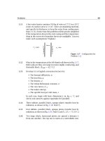
Figure 4.11 A general fin of variable cross section.
Fins of variable cross section
Let us consider what is involved is the design of a fin for which A and
P are functions of x. Such a fin is shown in Fig. 4.11. We restrict our
attention to fins for which

h(A/P)
k
 1 and
d(a/P)
d(x)
 1
so the heat flow will be approximately one-dimensional in x.
We begin the analysis, as always, with the First Law statement:
Q
net
= Q
cond
−Q
conv
=
dU
dt
or
7

kA(x +δx)
dT
dx




x=δx
−kA(x)
dT

dx




x


 
=
d
dx
kA(x)
dT
dx
δx
−
hP δx (T −T
∞
)
= ρcA(x)δx
dT
dt

 
=0, since steady
7
Note that we approximate the external area of the fin as horizontal when we write
it as Pδx. The actual area is negligibly larger than this in most cases. An exception
would be the tip of the fin in Fig. 4.11.

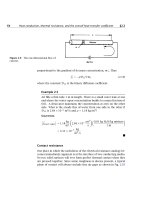
180 Analysis of heat conduction and some steady one-dimensional problems §4.5
Figure 4.12 A two-dimensional wedge-shaped fin.
Therefore,
d
dx

A(x)
d(T −T
∞
)
dx

−
hP
k
(T −T
∞
) = 0 (4.60)
If A(x) = constant, this reduces to Θ

−(mL)
2
Θ = 0, which is the straight
fin equation.
To see how eqn. (4.60) works, consider the triangular fin shown in
Fig. 4.12. In this case eqn. (4.60) becomes
d
dx

2δ


x
L

b
d(T −T
∞
)
dx

−
2
hb
k
(T −T
∞
) = 0
or
ξ
d
2
Θ
dξ
2
+
dΘ
dξ
−
hL
2

kδ

 
a kind
of (mL)
2
Θ = 0 (4.61)
This second-order linear differential equation is difficult to solve because
it has a variable coefficient. Its solution is expressible in Bessel functions:
Θ =
I
o

2

hLx/kδ

I
o

2

hL
2
/kδ

(4.62)
Fin design 181
where the modified Bessel function of the first kind, I
o

, can be looked up
in appropriate tables.
Rather than explore the mathematics of solving eqn. (4.60), we simply
show the result for several geometries in terms of the fin efficiency, η
f
,
in Fig. 4.13. These curves were given by Schneider [4.7]. Kraus, Aziz, and
Welty [4.8] provide a very complete discussion of fins and show a great
many additional efficiency curves.
Example 4.11
A thin brass pipe, 3 cm in outside diameter, carries hot water at 85
◦
C.
It is proposed to place 0.8 mm thick straight circular fins on the pipe
to cool it. The fins are 8 cm in diameter and are spaced 2 cm apart. It
is determined that
h will equal 20 W/m
2
K on the pipe and 15 W/m
2
K
on the fins, when they have been added. If T
∞
=22
◦
C, compute the
heat loss per meter of pipe before and after the fins are added.
Solution. Before the fins are added,
Q = π(0.03 m)(20 W/m
2

K)[(85 −22) K] = 199 W/m
where we set T
wall
− T
water
since the pipe is thin. Notice that, since
the wall is constantly heated by the water, we should not have a root-
temperature depression problem after the fins are added. Then we
can enter Fig. 4.13a with
r
2
r
1
= 2.67 and mL

L
P
=

hL
3
kA
=

15(0.04 −0.15)
3
125(0.025)(0.0008)
= 0.306
and we obtain η
f

= 89%. Thus, the actual heat transfer given by
Q
without fin
  
119 W/m

0.02 −0.0008
0.02


 
fraction of unfinned area
+0.89 [2π(0.04
2
−0.015
2
)]

 
area per fin (both sides), m
2

50
fins
m

15
W
m
2

K

[
(85 −22) K
]
so
Q
net
= 478 W/m = 4.02 Q
without fins
Figure 4.13 The efficiency of several fins with variable cross section.
182
Problems 183
Problems
4.1 Make a table listing the general solutions of all steady, unidi-
mensional constant-properties heat conduction problemns in
Cartesian, cylindrical and spherical coordinates, with and with-
out uniform heat generation. This table should prove to be a
very useful tool in future problem solving. It should include a
total of 18 solutions. State any restrictions on your solutions.
Do not include calculations.
4.2 The left side of a slab of thickness L is kept at 0
◦
C. The right
side is cooled by air at T
∞
◦
C blowing on it. h
RHS
is known. An

exothermic reaction takes place in the slab such that heat is
generated at A(T − T
∞
) W/m
3
, where A is a constant. Find a
fully dimensionless expression for the temperature distribu-
tion in the wall.
4.3 A long, wide plate of known size, material, and thickness L is
connected across the terminals of a power supply and serves
as a resistance heater. The voltage, current and T
∞
are known.
The plate is insulated on the bottom and transfers heat out
the top by convection. The temperature, T
tc
, of the botton
is measured with a thermocouple. Obtain expressions for (a)
temperature distribution in the plate; (b)
h at the top; (c) tem-
perature at the top. (Note that your answers must depend on
known information only.) [T
top
= T
tc
−EIL
2
/(2k ·volume)]
4.4 The heat tansfer coefficient,
h, resulting from a forced flow

over a flat plate depends on the fluid velocity, viscosity, den-
sity, specific heat, and thermal conductivity, as well as on the
length of the plate. Develop the dimensionless functional equa-
tion for the heat transfer coefficient (cf. Section 6.5).
4.5 Water vapor condenses on a cold pipe and drips off the bottom
in regularly spaced nodes as sketched in Fig. 3.9. The wave-
length of these nodes, λ, depends on the liquid-vapor density
difference, ρ
f
−ρ
g
, the surface tension, σ , and the gravity, g.
Find how λ varies with its dependent variables.
4.6 A thick film flows down a vertical wall. The local film velocity
at any distance from the wall depends on that distance, gravity,
the liquid kinematic viscosity, and the film thickness. Obtain
184 Chapter 4: Analysis of heat conduction and some steady one-dimensional problems
the dimensionless functional equation for the local velocity (cf.
Section 8.5).
4.7 A steam preheater consists of a thick, electrically conduct-
ing, cylindrical shell insulated on the outside, with wet stream
flowing down the middle. The inside heat transfer coefficient
is highly variable, depending on the velocity, quality, and so
on, but the flow temperature is constant. Heat is released at
˙
q J/m
3
s within the cylinder wall. Evaluate the temperature
within the cylinder as a function of position. Plot Θ against
ρ, where Θ is an appropriate dimensionless temperature and

ρ = r/r
o
. Use ρ
i
= 2/3 and note that Bi will be the parameter
of a family of solutions. On the basis of this plot, recommend
criteria (in terms of Bi) for (a) replacing the convective bound-
ary condition on the inside with a constant temperature condi-
tion; (b) neglecting temperature variations within the cylinder.
4.8 Steam condenses on the inside of a small pipe, keeping it at
a specified temperature, T
i
. The pipe is heated by electrical
resistance at a rate
˙
q W/m
3
. The outside temperature is T
∞
and
there is a natural convection heat transfer coefficient,
h around
the outside. (a) Derive an expression for the dimensionless
expression temperature distribution, Θ = (T −T
∞
)/(T
i
−T
∞
),

as a function of the radius ratios, ρ = r/r
o
and ρ
i
= r
i
/r
o
;
a heat generation number, Γ =
˙
qr
2
o
/k(T
i
− T
∞
); and the Biot
number. (b) Plot this result for the case ρ
i
= 2/3, Bi = 1, and
for several values of Γ . (c) Discuss any interesting aspects of
your result.
4.9 Solve Problem 2.5 if you have not already done so, putting
it in dimensionless form before you begin. Then let the Biot
numbers approach infinity in the solution. You should get the
same solution we got in Example 2.5, using b.c.’s of the first
kind. Do you?
4.10 Complete the algebra that is missing between eqns. (4.30) and

eqn. (4.31b) and eqn. (4.41).
4.11 Complete the algebra that is missing between eqns. (4.30) and
eqn. (4.31a) and eqn. (4.48).
Problems 185
4.12 Obtain eqn. (4.50) from the general solution for a fin [eqn. (4.35)],
using the b.c.’s T(x = 0) = T
0
and T(x = L) = T
∞
. Comment
on the significance of the computation.
4.13 What is the minimum length, l, of a thermometer well neces-
sary to ensure an error less than 0.5% of the difference between
the pipe wall temperature and the temperature of fluid flowing
in a pipe? The well consists of a tube with the end closed. It
hasa2cmO.D. and a 1.88 cm I.D. The material is type 304
stainless steel. Assume that the fluid is steam at 260
◦
C and
that the heat transfer coefficient between the steam and the
tube wall is 300 W/m
2
K. [3.44 cm.]
4.14 Thin fins with a 0.002 m by 0.02 m rectangular cross section
and a thermal conductivity of 50 W/m·K protrude from a wall
and have
h  600 W/m
2
K and T
0

= 170
◦
C. What is the heat
flow rate into each fin and what is the effectiveness? T
∞
=
20
◦
C.
4.15 A thin rod is anchored at a wall at T = T
0
on one end and is
insulated at the other end. Plot the dimensionless temperature
distribution in the rod as a function of dimensionless length:
(a) if the rod is exposed to an environment at T
∞
through a
heat transfer coefficient; (b) if the rod is insulated but heat is
removed from the fin material at the unform rate −
˙
q =
hP(T
0
−
T
∞
)/A. Comment on the implications of the comparison.
4.16 A tube of outside diameter d
o
and inside diameter d

i
carries
fluid at T = T
1
from one wall at temperature T
1
to another
wall a distance L away, at T
r
. Outside the tube h
o
is negligible,
and inside the tube
h
i
is substantial. Treat the tube as a fin
and plot the dimensionless temperature distribution in it as a
function of dimensionless length.
4.17 (If you have had some applied mathematics beyond the usual
two years of calculus, this problem will not be difficult.) The
shape of the fin in Fig. 4.12 is changed so that A(x) = 2δ(x/L)
2
b
instead of 2δ(x/L)b. Calculate the temperature distribution
and the heat flux at the base. Plot the temperature distribution
and fin thickness against x/L. Derive an expression for η
f
.
186 Chapter 4: Analysis of heat conduction and some steady one-dimensional problems
4.18 Work Problem 2.21, if you have not already done so, nondi-

mensionalizing the problem before you attempt to solve it. It
should now be much simpler.
4.19 One end of a copper rod 30 cm long is held at 200
◦
C, and the
other end is held at 93
◦
C. The heat transfer coefficient in be-
tween is 17 W/m
2
K (including both convection and radiation).
If T
∞
=38
◦
C and the diameter of the rod is 1.25 cm, what is
the net heat removed by the air around the rod? [19.13 W.]
4.20 How much error will the insulated-tip assumption give rise to
in the calculation of the heat flow into the fin in Example 4.8?
4.21 A straight cylindrical fin 0.6 cm in diameter and 6 cm long
protrudes from a magnesium block at 300
◦
C. Air at 35
◦
Cis
forced past the fin so that
h is 130 W/m
2
K. Calculate the heat
removed by the fin, considering the temperature depression of

the root.
4.22 Work Problem 4.19 considering the temperature depression in
both roots. To do this, find mL for the two fins with insulated
tips that would give the same temperature gradient at each
wall. Base the correction on these values of mL.
4.23 A fin of triangular axial section (cf. Fig. 4.12) 0.1 m in length
and 0.02 m wide at its base is used to extend the surface area
of a 0.5% carbon steel wall. If the wall is at 40
◦
C and heated
gas flows past at 200
◦
C(h = 230 W/m
2
K), compute the heat
removed by the fin per meter of breadth, b, of the fin. Neglect
temperature distortion at the root.
4.24 Consider the concrete slab in Example 2.1. Suppose that the
heat generation were to cease abruptly at time t = 0 and the
slab were to start cooling back toward T
w
. Predict T = T
w
as a
function of time, noting that the initial parabolic temperature
profile can be nicely approximated as a sine function. (Without
the sine approximation, this problem would require the series
methods of Chapter 5.)
4.25 Steam condenses ina2cmI.D. thin-walled tube of 99% alu-
minum at 10 atm pressure. There are circular fins of constant

thickness, 3.5 cm in diameter, every 0.5 cm on the outside. The
Problems 187
fins are 0.8 mm thick and the heat transfer coefficient from
them
h = 6 W/m
2
K (including both convection and radiation).
What is the mass rate of condensation if the pipe is 1.5 m in
length, the ambient temperature is 18
◦
C, and h for condensa-
tion is very large? [
˙
m
cond
= 0.802 kg/hr.]
4.26 How long must a copper fin, 0.4 cm in diameter, be if the tem-
perature of its insulated tip is to exceed the surrounding air
temperature by 20% of (T
0
− T
∞
)? T
air
= 20
◦
C and h = 28
W/m
2
K (including both convection and radiation).

4.27 A 2 cm ice cube sits on a shelf of aluminum rods, 3 mm in diam-
eter, in a refrigerator at 10
◦
C. How rapidly, in mm/min, does
the ice cube melt through the wires if
h at the surface of the
wires is 10 W/m
2
K (including both convection and radiation).
Be sure that you understand the physical mechanism before
you make the calculation. Check your result experimentally.
h
sf
= 333, 300 J/kg.
4.28 The highest heat flux that can be achieved in nucleate boil-
ing (called q
max
—see the qualitative discussion in Section 9.1)
depends upon ρ
g
, the saturated vapor density; h
fg
, the la-
tent heat vaporization; σ , the surface tension; a characteristic
length, l; and the gravity force per unit volume, g(ρ
f
− ρ
g
),
where ρ

f
is the saturated liquid density. Develop the dimen-
sionless functional equation for q
max
in terms of dimension-
less length.
4.29 You want to rig a handle for a door in the wall of a furnace. The
door is at 160
◦
C. You consider bending a 16 in. length of ¼ in.
0.5% carbon steel rod into a U-shape and welding the ends to
the door. Surrounding air at 24
◦
C will cool the handle (h = 12
W/m
2
K including both convection and radiation). What is the
coolest temperature of the handle? How close to the door can
you grasp it without being burned? How might you improve
the handle?
4.30 A 14 cm long by 1 cm square brass rod is supplied with 25 W at
its base. The other end is insulated. It is cooled by air at 20
◦
C,
with
h = 68 W/m
2
K. Develop a dimensionless expression for
Θ as a function of ε
f

and other known information. Calculate
the base temperature.
188 Chapter 4: Analysis of heat conduction and some steady one-dimensional problems
4.31 A cylindrical fin has a constant imposed heat flux of q
1
at one
end and q
2
at the other end, and it is cooled convectively along
its length. Develop the dimensionless temperature distribu-
tion in the fin. Specialize this result for q
2
= 0 and L →∞, and
compare it with eqn. (4.50).
4.32 A thin metal cylinder of radius r
o
serves as an electrical re-
sistance heater. The temperature along an axial line in one
side is kept at T
1
. Another line, θ
2
radians away, is kept at
T
2
. Develop dimensionless expressions for the temperature
distributions in the two sections.
4.33 Heat transfer is augmented, in a particular heat exchanger,
with a field of 0.007 m diameter fins protruding 0.02 m into a
flow. The fins are arranged in a hexagonal array, with a mini-

mum spacing of 1.8 cm. The fins are bronze, and
h
f
around
the fins is 168 W/m
2
K. On the wall itself, h
w
is only 54 W/m
2
K.
Calculate
h
eff
for the wall with its fins. (h
eff
= Q
wall
divided by
A
wall
and [T
wall
−T
∞
].)
4.34 Evaluate d(tanh x)/dx.
4.35 An engineer seeks to study the effect of temperature on the
curing of concrete by controlling the temperature of curing in
the following way. A sample slab of thickness L is subjected

to a heat flux, q
w
, on one side, and it is cooled to temperature
T
1
on the other. Derive a dimensionless expression for the
steady temperature in the slab. Plot the expression and offer
a criterion for neglecting the internal heat generation in the
slab.
4.36 Develop the dimensionless temperature distribution in a spher-
ical shell with the inside wall kept at one temperature and the
outside wall at a second temperature. Reduce your solution
to the limiting cases in which r
outside
 r
inside
and in which
r
outside
is very close to r
inside
. Discuss these limits.
4.37 Does the temperature distribution during steady heat transfer
in an object with b.c.’s of only the first kind depend on k?
Explain.
4.38 A long, 0.005 m diameter duralumin rod is wrapped with an
electrical resistor over 3 cm of its length. The resistor imparts