Biosignal and Biomedical Image Processing phần 7 pps

Advanced Signal Processing 237
V′(t) = V
s
k/4R [cos(2ω
c
t +θ+ω
s
t) + cos(2ω
c
t +θ−ω
s
t)
+ cos(ω
s
t +θ) + cos(ω
s
t −θ)] (24)
The spectrum of V′(t) is shown in Figure 8.13. Note that the phase angle,
θ, would have an influence on the magnitude of the signal, but not its frequency.
After lowpass digital filtering the higher frequency terms, ω
c
t ±ω
s
will be
reduced to near zero, so the output, V
out
(t), becomes:
V
out
(t) = A(t)cosθ=(V
s

k/2R)cosθ (25)
Since cos θ is a constant, the output of the phase sensitive detector is the
demodulated signal, A(t), multiplied by this constant. The term phase sensitive
is derived from the fact that the constant is a function of the phase difference,
θ, between V
c
(t) and V
in
(t). Note that while θ is generally constant, any shift in
phase between the two signals will induce a change in the output signal level,
so this approach could also be used to detect phase changes between signals of
constant amplitude.
The multiplier operation is similar to the sampling process in that it gener-
ates additional frequency components. This will reduce the influence of low
frequency noise since it will be shifted up to near the carrier frequency. For
example, consider the effect of the multiplier on 60 Hz noise (or almost any
noise that is not near to the carrier frequency). Using the principle of superposit-
ion, only the noise component needs to be considered. For a noise component
at frequency, ω
n
(V
in
(t)
NOISE
= V
n
cos (ω
n
t)). After multiplication the contribution
at V′(t) will be:

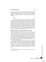
F
IGURE
8.13 Frequency spectrum of the signal created by multiplying the V
in
(t)
by the carrier frequency. After lowpass filtering, only the original low frequency
signal at ω
s
will remain.
TLFeBOOK
238 Chapter 8
V
in
(t)
NOISE
= V
n
[cos(ω
c
t +ω
n
t) + cos(ω
c
t +ω
s
t)] (26)
and the new, complete spectrum for V′(t) is shown in Figure 8.14.
The only frequencies that will not be attenuated in the input signal, V
in
(t),

are those around the carrier frequency that also fall within the bandwidth of the
lowpass filter. Another way to analyze the noise attenuation characteristics of
phase sensitive detection is to view the effect of the multiplier as shifting the
lowpass filter’s spectrum to be symmetrical about the carrier frequency, giving
it the form of a narrow bandpass filter (Figure 8.15). Not only can extremely
narrowband bandpass filters be created this way (simply by having a low cutoff
frequency in the lowpass filter), but more importantly the center frequency of
the effective bandpass filter tracks any changes in the carrier frequency. It is
these two features, narrowband filtering and tracking, that give phase sensitive
detection its signal processing power.
MATLAB Implementation
Phase sensitive detection is implemented in MATLAB using simple multiplica-
tion and filtering. The application of a phase sensitive detector is given in Exam-
F
IGURE
8.14 Frequency spectrum of the signal created by multiplying V
in
(t) in-
cluding low frequency noise by the carrier frequency. The low frequency noise is
shifted up to ± the carrier frequency. After lowpass filtering, both the noise and
higher frequency signal are greatly attenuated, again leaving only the original low
frequency signal at ω
s
remaining.
TLFeBOOK
Advanced Signal Processing 239
F
IGURE
8.15 Frequency characteristics of a phase sensitive detector. The fre-
quency response of the lowpass filter (solid line) is effectively “reflected” about

the carrier frequency, fc, producing the effect of a narrowband bandpass filter
(dashed line). In a phase sensitive detector the center frequency of this virtual
bandpass filter tracks the carrier frequency.
ple 8.6 below. A carrier sinusoid of 250 Hz is modulated with a sawtooth wave
with a frequency of 5 Hz. The AM signal is buried in noise that is 3.16 times
the signal (i.e., SNR = -10 db).
Example 8.6 Phase Sensitive Detector. This example uses a phase sensi-
tive detection to demodulate the AM signal and recover the signal from noise.
The filter is chosen as a second-order Butterworth lowpass filter with a cutoff
frequency set for best noise rejection while still providing reasonable fidelity to
the sawtooth waveform. The example uses a sampling frequency of 2 kHz.
% Example 8.6 and Figure 8.16 Phase Sensitive Detection
%
% Set constants
close all; clear all;
fs = 2000; % Sampling frequency
f = 5; % Signal frequency
fc = 250; % Carrier frequency
N = 2000; % Use 1 sec of data
t = (1:N)/fs; % Time axis for plotting
wn = .02; % PSD lowpass filter cut-
% off frequency
[b,a] = butter(2,wn); % Design lowpass filter
%
TLFeBOOK
240 Chapter 8
F
IGURE
8.16 Application of phase sensitive detection to an amplitude-modulated
signal. The AM signal consisted of a 250 Hz carrier modulated by a 5 Hz sawtooth

(upper graph). The AM signal is mixed with white noise (SNR =−10db, middle
graph). The recovered signal shows a reduction in the noise (lower graph).
% Generate AM signal
w = (1:N)* 2*pi*fc/fs; % Carrier frequency =
% 250 Hz
w1 = (1:N)*2*pi*f/fs; % Signal frequency = 5Hz
vc = sin(w); % Define carrier
vsig = sawtooth(w1,.5); % Define signal
vm = (1 ؉ .5 * vsig) .* vc; % Create modulated signal
TLFeBOOK
Advanced Signal Processing 241
% with a Modulation
% constant = 0.5
subplot(3,1,1);
plot(t,vm,’k’); % Plot AM Signal
axis, label,title
%
% Add noise with 3.16 times power (10 db) of signal for SNR of
% -10 db
noise = randn(1,N);
scale = (var(vsig)/var(noise)) * 3.16;
vm = vm ؉ noise * scale; % Add noise to modulated
% signal
subplot(3,1,2);
plot(t,vm,’k’); % Plot AM signal
axis, label,title
% Phase sensitive detection
ishift = fix(.125 * fs/fc); % Shift carrier by 1/4
vc = [vc(ishift:N) vc(1:ishift-1)]; % period (45 deg) using
% periodic shift

v1 = vc .* vm; % Multiplier
vout = filter(b,a,v1); % Apply lowpass filter
subplot(3,1,3);
plot(t,vout,’k’); % Plot AM Signal
axis, label,title
The lowpass filter was set to a cutoff frequency of 20 Hz (0.02 * f
s
/2) as
a compromise between good noise reduction and fidelity. (The fidelity can be
roughly assessed by the sharpness of the peaks of the recovered sawtooth wave.)
A major limitation in this process were the characteristics of the lowpass filter:
digital filters do not perform well at low frequencies. The results are shown in
Figure 8.16 and show reasonable recovery of the demodulated signal from the
noise.
Even better performance can be obtained if the interference signal is nar-
rowband such as 60 Hz interference. An example of using phase sensitive detec-
tion in the presence of a strong 60 Hz signal is given in Problem 6 below.
PROBLEMS
1. Apply the Wiener-Hopf approach to a signal plus noise waveform similar
to that used in Example 8.1, except use two sinusoids at 10 and 20 Hz in 8 db
noise. Recall, the function
sig_noise
provides the noiseless signal as the third
output to be used as the desired signal. Apply this optimal filter for filter lengths
of 256 and 512.
TLFeBOOK
242 Chapter 8
2. Use the LMS adaptive filter approach to determine the FIR equivalent to
the linear process described by the digital transfer function:
H(z) =

0.2 + 0.5z
−1
1 − 0.2z
−1
+ 0.8z
−2
As with Example 8.2, plot the magnitude digital transfer function of the
“unknown” system, H(z), and of the FIR “matching” system. Find the transfer
function of the IIR process by taking the square of the magnitude of
fft(b,n)./fft(a,n)
(or use
freqz
). Use the MATLAB function
filtfilt
to produce the output of the IIR process. This routine produces no time delay
between the input and filtered output. Determine the approximate minimum
number of filter coefficients required to accurately represent the function above
by limiting the coefficients to different lengths.
3. Generate a 20 Hz interference signal in noise with and SNR + 8 db; that is,
the interference signal is 8 db stronger that the noise. (Use
sig_noise
with an
SNR of +8. ) In this problem the noise will be considered as the desired signal.
Design an adaptive interference filter to remove the 20 Hz “noise.” Use an FIR
filter with 128 coefficients.
4. Apply the ALE filter described in Example 8.3 to a signal consisting of two
sinusoids of 10 and 20 Hz that are present simultaneously, rather that sequen-
tially as in Example 8.3. Use a FIR filter lengths of 128 and 256 points. Evaluate
the influence of modifying the delay between 4 and 18 samples.
5. Modify the code in Example 8.5 so that the reference signal is correlat-

ed with, but not the same as, the interference data. This should be done by con-
volving the reference signal with a lowpass filter consisting of 3 equal weights;
i.e:
b = [ 0.333 0.333 0.333].
For this more realistic scenario, note the degradation in performance as
compared to Example 8.5 where the reference signal was identical to the noise.
6. Redo the phase sensitive detector in Example 8.6, but replace the white
noise with a 60 Hz interference signal. The 60 Hz interference signal should
have an amplitude that is 10 times that of the AM signal.
TLFeBOOK
9
Multivariate Analyses:
Principal Component Analysis
and Independent Component Analysis
INTRODUCTION
Principal component analysis and independent component analysis fall within a
branch of statistics known as multivariate analysis. As the name implies, multi-
variate analysis is concerned with the analysis of multiple variables (or measure-
ments), but treats them as a single entity (for example, variables from multiple
measurements made on the same process or system). In multivariate analysis,
these multiple variables are often represented as a single vector variable that
includes the different variables:
x = [x
1
(t), x
2
(t) x
m
(t)]
T

For 1 ≤ m ≤ M (1)
The ‘T’ stands for transposed and represents the matrix operation of
switching rows and columns.* In this case, x is composed of M variables, each
containing N (t = 1, ,N ) observations. In signal processing, the observations
are time samples, while in image processing they are pixels. Multivariate data,
as represented by x above can also be considered to reside in M-dimensional
space, where each spatial dimension contains one signal (or image).
In general, multivariate analysis seeks to produce results that take into
*Normally, all vectors including these multivariate variables are taken as column vectors, but to
save space in this text, they are often written as row vectors with the transpose symbol to indicate
that they are actually column vectors.
243
TLFeBOOK
244 Chapter 9
account the relationship between the multiple variables as well as within the
variables, and uses tools that operate on all of the data. For example, the covari-
ance matrix described in Chapter 2 (Eq. (19), Chapter 2, and repeated in Eq.
(4) below) is an example of a multivariate analysis technique as it includes
information about the relationship between variables (their covariance) and in-
formation about the individual variables (their variance). Because the covariance
matrix contains information on both the variance within the variables and the
covariance between the variables, it is occasionally referred to as the variance–
covariance matrix.
A major concern of multivariate analysis is to find transformations of the
multivariate data that make the data set smaller or easier to understand. For
example, is it possible that the relevant information contained in a multidimen-
sional variable could be expressed using fewer dimensions (i.e., variables) and
might the reduced set of variables be more meaningful than the original data
set? If the latter were true, we would say that the more meaningful variables
were hidden, or latent, in the original data; perhaps the new variables better

represent the underlying processes that produced the original data set. A bio-
medical example is found in EEG analysis where a large number of signals are
acquired above the region of the cortex, yet these multiple signals are the result
of a smaller number of neural sources. It is the signals generated by the neural
sources—not the EEG signals per se—that are of interest.
In transformations that reduce the dimensionality of a multi-variable data
set, the idea is to transform one set of variables into a new set where some of
the new variables have values that are quite small compared to the others. Since
the values of these variables are relatively small, they must not contribute very
much information to the overall data set and, hence, can be eliminated.* With
the appropriate transformation, it is sometimes possible to eliminate a large
number of variables that contribute only marginally to the total information.
The data transformation used to produce the new set of variables is often
a linear function since linear transformations are easier to compute and their
results are easier to interpret. A linear transformation can be represent mathe-
matically as:
y
i
(t) =
∑
M
j=1
w
ij
x
j
(t) i = 1, N (2)
where w
ij
is a constant coefficient that defines the transformation.

*Evaluating the significant of a variable by the range of its values assumes that all the original
variables have approximately the same range. If not, some form of normalization should be applied
to the original data set.
TLFeBOOK
PCA and ICA 245
Since this transformation is a series of equations, it can be equivalently
expressed using the notation of linear algebra:
ͫ
y
1
(t)
y
2
(t)
Ӈ
y
M
(t)
ͬ
= W
ͫ
x
1
(t)
x
2
(t)
Ӈ
x
M

(t)
ͬ
(3)
As a linear transformation, this operation can be interpreted as a rotation
and possibly scaling of the original data set in M-dimensional space. An exam-
ple of how a rotation of a data set can produce a new data set with fewer major
variables is shown in Figure 9.1 for a simple two-dimensional (i.e., two vari-
able) data set. The original data set is shown as a plot of one variable against
the other, a so-called scatter plot, in Figure 9.1A. The variance of variable x
1
is
0.34 and the variance of x
2
is 0.20. After rotation the two new variables, y
1
and
y
2
have variances of 0.53 and 0.005, respectively. This suggests that one vari-
able, y
1
, contains most of the information in the original two-variable set. The
F
IGURE
9.1 A data set consisting of two variables before (left graph) and after
(right graph) linear rotation. The rotated data set still has two variables, but the
variance on one of the variables is quite small compared to the other.
TLFeBOOK
246 Chapter 9
goal of this approach to data reduction is to find a matrix W that will produce

such a transformation.
The two multivariate techniques discussed below, principal component
analysis and independent component analysis, differ in their goals and in the
criteria applied to the transformation. In principal component analysis, the object
is to transform the data set so as to produce a new set of variables (termed
principal components) that are uncorrelated. The goal is to reduce the dimen-
sionality of the data, not necessarily to produce more meaningful variables. We
will see that this can be done simply by rotating the data in M-dimensional
space. In independent component analysis, the goal is a bit more ambitious:
to find new variables (components) that are both statistically independent and
nongaussian.
PRINCIPAL COMPONENT ANALYSIS
Principal component analysis (PCA) is often referred to as a technique for re-
ducing the number of variables in a data set without loss of information, and as
a possible process for identifying new variables with greater meaning. Unfortu-
nately, while PCA can be, and is, used to transform one set of variables into
another smaller set, the newly created variables are not usually easy to interpret.
PCA has been most successful in applications such as image compression where
data reduction—and not interpretation—is of primary importance. In many ap-
plications, PCA is used only to provide information on the true dimensionality
of a data set. That is, if a data set includes M variables, do we really need all
M variables to represent the information, or can the variables be recombined
into a smaller number that still contain most of the essential information (John-
son, 1983)? If so, what is the most appropriate dimension of the new data set?
PCA operates by transforming a set of correlated variables into a new set
of uncorrelated variables that are called the principal components. Note that if
the variables in a data set are already uncorrelated, PCA is of no value. In
addition to being uncorrelated, the principal components are orthogonal and are
ordered in terms of the variability they represent. That is, the first principle
component represents, for a single dimension (i.e., variable), the greatest amount

of variability in the original data set. Each succeeding orthogonal component
accounts for as much of the remaining variability as possible.
The operation performed by PCA can be described in a number of ways,
but a geometrical interpretation is the most straightforward. While PCA is appli-
cable to data sets containing any number of variables, it is easier to describe
using only two variables since this leads to readily visualized graphs. Figure
9.2A shows two waveforms: a two-variable data set where each variable is a
different mixture of the same two sinusoids added with different scaling factors.
A small amount of noise was also added to each waveform (see Example 9.1).
TLFeBOOK
PCA and ICA 247
F
IGURE
9.2 (A) Two waveforms made by mixing two sinusoids having different
frequencies and amplitudes, then adding noise to the two mixtures. The resultant
waveforms can be considered related variables since they both contain informa-
tion from the same two sources. (B) The scatter plot of the two variables (or
waveforms) was obtained by plotting one variable against the other for each point
in time (i.e., each data sample). The correlation between the two samples (r =
0.77) can be seen in the diagonal clustering of points.
Since the data set was created using two separate sinusoidal sources, it should
require two spatial dimensions. However, since each variable is composed of
mixtures of the two sources, the variables have a considerable amount of covari-
ance, or correlation.* Figure 9.2B is a scatter plot of the two variables, a plot
of x
1
against x
2
for each point in time, and shows the correlation between the
variabl es as a diagona l sp re ad of the data po in ts. (T he c orrelation be twe en the two

variables is 0.77.) Thus, knowledge of the x value gives information on the
*Recall that covariance and correlation differ only in scaling. Definitions of these terms are given
in Chapter 2 and are repeated for covariance below.
TLFeBOOK
248 Chapter 9
range of possible y values and vice versa. Note that the x value does not
uniquely determine the y value as the correlation between the two variables is
less than one. If the data were uncorrelated, the x value would provide no infor-
mation on possible y values and vice versa. A scatter plot produced for such
uncorrelated data would be roughly symmetrical with respect to both the hori-
zontal and vertical axes.
For PCA to decorrelate the two variables, it simply needs to rotate the
two-variable data set until the data points are distributed symmetrically about
the mean. Figure 9.3B shows the results of such a rotation, while Figure 9.3A
plots the time response of the transformed (i.e., rotated) variables. In the decor-
related condition, the variance is maximally distributed along the two orthogonal
axes. In general, it may be also necessary to center the data by removing the
means before rotation. The original variables plotted in Figure 9.2 had zero
means so this step was not necessary.
While it is common in everyday language to take the word uncorrelated
as meaning unrelated (and hence independent), this is not the case in statistical
analysis, particularly if the variables are nonlinear. In the statistical sense, if two
F
IGURE
9.3 (A) Principal components of the two variables shown in Figure 9.2.
These were produced by an orthogonal rotation of the two variables. (B) The
scatter plot of the rotated principal components. The symmetrical shape of the
data indicates that the two new components are uncorrelated.
TLFeBOOK
PCA and ICA 249

(or more) variables are independent they will also be uncorrelated, but the re-
verse is not generally true. For example, the two variables plotted as a scatter
plot in Figure 9.4 are uncorrelated, but they are highly related and not indepen-
dent. They are both generated by a single equation, the equation for a circle with
noise added. Many other nonlinear relationships (such as the quadratic function)
can generate related (i.e., not independent) variables that are uncorrelated. Con-
versely, if the variables have a Gaussian distribution (as in the case of most
noise), then when they are uncorrelated they are also independent. Note that
most signals do not have a Gaussian distribution and therefore are not likely to
be independent after they have been decorrelated using PCA. This is one of the
reasons why the principal components are not usually meaningful variables:
they are still mixtures of the underlying sources. This inability to make two
signals independent through decorrelation provides the motivation for the meth-
odology k nown as independent com ponen t analysis described later in this c hapte r.
If only two variables are involved, the rotation performed between Figure
9.2 and Figure 9.3 could be done by trial and error: simply rotate the data until
F
IGURE
9.4 Time and scatter plots of two variables that are uncorrelated, but not
independent. In fact, the two variables were generated by a single equation for a
circle with added noise.
TLFeBOOK
250 Chapter 9
the covariance (or correlation) goes to zero. An example of this approach is
given as an exercise in the problems. A better way to achieve zero correlation
is to use a technique from linear algebra that generates a rotation matrix that
reduces the covariance to zero. A well-known technique exists to reduce a ma-
trix that is positive-definite (as is the covariance matrix) into a diagonal matrix
by pre- and post-multiplication with an orthonormal matrix (Jackson, 1991):
U′SU = D (4)

where S is the m-by-m covariance matrix, D is a diagonal matrix, and U is an
orthonormal matrix that does the transformation. Recall that a diagonal matrix
has zeros for the off-diagonal elements, and it is the off-diagonal elements that
correspond to covariance in the covariance matrix (Eq. (19) in Chapter 2 and
repeated as Eq. (5) below). The covariance matrix is defined by:
S =
ͫ
σ
1,1
σ
1,2

σ
1,N
σ
2,1
σ
2,2

σ
2,N
ӇӇO Ӈ
σ
N,1
σ
N,2

σ
N,N
ͬ

(5)
Hence, the rotation implied by U will produce a new covariance matrix,
D, that has zero covariance. The diagonal elements of D are the variances of
the new data, more generally known as the characteristic roots, or eigenvalues,
of S: λ
1
, λ
2
, λ
n
. The columns of U are the characteristic vectors, or eigenvec-
tors u
1
, u
2
, u
n
. Again, the eigenvalues of the new covariance matrix, D, cor-
respond to the variances of the rotated variables (now called the principle com-
ponents). Accordingly, these eigenvalues (variances) can be used to determine
what percentage of the total variance (which is equal to the sum of all eigenval-
ues) a given principal component represents. As shown below, this is a measure
of the associated principal component’s importance, at least with regard to how
much of the total information it represents.
The eigenvalues or roots can be solved by the following determinant equa-
tion:
det*S −λI* = 0(6)
where I is the identity matrix. After solving for λ, the eigenvectors can be
solved using the equation:
det*S −λI*b

i
= 0(7)
where the eigenvectors are obtained from b
i
by the equation
u
i
= b
i
'
√
b′
i
b
i
(8)
TLFeBOOK
PCA and ICA 251
This approach can be carried out by hand for two or three variables, but
is very tedious for more variables or long data sets. It is much easier to use
singular value composition which has the advantage of working directly from
the data matrix and can be done in one step. Moreover, singular value decompo-
sition can be easily implemented with a single function call in MATLAB. Sin-
gular value decomposition solves an equation similar to Eq. (4), specifically:
X = U*D
1/2
U′ (9)
In the case of PCA, X is the data matrix that is decomposed into (1) D,
the diagonal matrix that contains, in this case, the square root of the eigenvalues;
and (2) U, the principle components matrix. An example of this approach is

given in the next section on MATLAB Implementation.
Order Selection
The eigenvalues describe how much of the variance is accounted for by the
associated principal component, and when singular value decomposition is used,
these eigenvalues are ordered by size; that is: λ
1
>λ
2
>λ
3
>λ
M
. They can
be very helpful in determining how many of the components are really signifi-
cant and how much the data set can be reduced. Specifically, if several eigenval-
ues are zero or close to zero, then the associated principal components contribute
little to the data and can be eliminated. Of course, if the eigenvalues are identi-
cally zero, then the associated principal component should clearly be eliminated,
but where do you make the cut when the eigenvalues are small, but nonzero?
There are two popular methods for determining eigenvalue thresholds. (1) Take
the sum of all eigenvectors (which must account for all the variance), then delete
those eigenvalues that fall below some percentage of that sum. For example, if
you want the remaining variables to account for 90% of the variance, then chose
a cutoff eigenvalue where the sum of all lower eigenvalues is less than 10% of
the total eigenvalue sum. (2) Plot the eigenvalues against the order number, and
look for breakpoints in the slope of this curve. Eigenvalues representing noise
should not change much in value and, hence, will plot as a flatter slope when
plotted against eigenvalue number (recall the eigenvalues are in order of large
to small). Such a curve was introduced in Chapter 5 and is known as the scree
plot (see Figure 5.6 D) These approaches are explored in the first example of

the following section on MATLAB Implementation.
MATLAB Implementation
Data Rotation
Many multivariate techniques rotate the data set as part of their operation. Im-
aging also uses data rotation to change the orientation of an object or image.
TLFeBOOK
252 Chapter 9
From basic trigonometry, it is easy to show that, in two dimensions, rotation of
a data point (x1, y1) can be achieved by multiplying the data points by the sines
and cosines of the rotation angle:
y
2
= y
1
cos(θ) + x
1
sin(θ)(10)
x
2
= y
1
(−sin(θ)) + x
1
cos(θ)(11)
where θ is the angle through which the data set is rotated in radians. Using
matrix notation, this operation can be done by multiplying the data matrix by a
rotation matrix:
R =
ͫ
cos(θ)

−sin(θ)
sin(θ)
cos(θ)
ͬ
(12)
This is the strategy used by the routine
rotation
given in Example 9.1
below. The generalization of this approach to three or more dimensions is
straightforward. In PCA, the rotation is done by the algorithm as described
below so explicit rotation is not required. (Nonetheless, it is required for one of
the problems at the end of this chapter, and later in image processing.) An
example of the application of rotation in two dimensions is given in the
example.
Example 9.1 This example generate two cycles of a sine wave and rotate
the wave by 45 deg.
Solution: The routine below uses the function
rotation
to perform the
rotation
. This function operates only on two-dimensional data. In addition to
multiplying the data set by the matrix in Eq. (12), the function
rotation
checks
the input matrix and ensures that it is in the right orientation for rotation with
the variables as columns of the data matrix. (It assumes two-dimensional data,
so the number of columns, i.e., number of variables, should be less than the
number of rows.)
% Example 9.1 and Figure 9.5
% Example of data rotation

% Create a two variable data set of y = sin (x)
% then rotate the data set by an angle of 45 deg
%
clear all; close all;
N = 100; % Variable length
x(1,:) = (1:N)/10; % Create a two variable data
x(2,:) = sin(x(1,:)*4*pi/10); % set: x1 linear; x2 =
% sin(x1)—two periods
plot(x(1,:),x(2,:),’*k’ ); % Plot data set
xlabel(’x1’); ylabel(’x2’);
phi = 45*(2*pi/360); % Rotation angle equals 45 deg
TLFeBOOK
PCA and ICA 253
F
IGURE
9.5 A two-cycle sine wave is rotated 45 deg. using the function
rota-
tion
that implements Eq. (12).
y = rotation(x,phi); % Rotate
hold on;
plot(y(1,:),y(2,:),’xk’); % Plot rotated data
The rotation is performed by the function
rotation
following Eq. (12).
% Function rotation
% Rotates the first argument by an angle phi given in the second
% argument function out = rotate(input,phi)
% Input variables
% input A matrix of the data to be rotated

phi The rotation angle in radians
% Output variables
% out The rotated data
%
[r c] = size(input);
if r < c % Check input format and
TLFeBOOK
254 Chapter 9
input = input’; % transpose if necessary
transpose_flag = ’y’;
end
% Set up rotation matrix
R = [cos(phi) sin(phi); -sin(phi) cos(phi)];
out = input * R; % Rotate input
if transpose_flag == ’y’ % Restore original input format
out = out’;
end
Principal Component Analysis Evaluation
PCA can be implemented using singular value decomposition. In addition, the
MATLAB Statistics Toolbox has a special program,
princomp
, but this just
implements the singular value decomposition algorithm. Singular value decom-
position of a data array,
X
, uses:
[V,D,U] = svd(X);
where
D
is a diagonal matrix containing the eigenvalues and

V
contains the
principal components in columns. The eigenvalues can be obtained from
D
using
the
diag
command:
eigen = diag(D);
Referring to Eq. (9), these values will actually be the square root of the
eigenvalues, λ
i
. If the eigenvalues are used to measure the variance in the rotated
principal components, they also need to be scaled by the number of points.
It is common to normalize the principal components by the eigenvalues
so that different components can be compared. While a number of different
normalizing schemes exist, in the examples here, we multiply the eigenvector
by the square root of the associated eigenvalue since this gives rise to principal
components that have the same value as a rotated data array (See Problem 1).
Example 9.2 Generate a data set with five variables, but from only two
sources and noise. Compute the principal components and associated eigenval-
ues using singular value decomposition. Compute the eigenvalue ratios and gen-
erate the scree plot. Plot the significant principal components.
% Example 9.2 and Figures 9.6, 9.7, and 9.8
% Example of PCA
% Create five variable waveforms from only two signals and noise
% Use this in PCA Analysis
%
% Assign constants
TLFeBOOK

PCA and ICA 255
F
IGURE
9.6 Plot of eigenvalue against component number, the scree plot. Since
the eigenvalue represents the variance of a given component, it can be used as
a measure of the amount of information the associated component represents. A
break is seen at 2, suggesting that only the first two principal components are
necessary to describe most of the information in the data.
clear all; close all;
N = 1000; % Number points (4 sec of
% data)
fs = 500; % Sample frequency
w = (1:N) * 2*pi/fs; % Normalized frequency
% vector
t = (1:N);*IH26* % Time vector for plotting
%
% Generate data
x = .75 *sin(w*5); % One component a sine
y = sawtooth(w*7,.5); % One component a sawtooth
%
% Combine data in different proportions
D(1,:) = .5*y ؉ .5*x ؉ .1*rand(1,N);
D(2,:) = .2*y ؉ .7*x ؉ .1*rand(1,N);
D(3,:) = .7*y ؉ .2*x ؉ .1*rand(1,N);
D(4,:) = 6*y ؉ 24*x ؉ .2*rand(1,N);
D(5,:) = .6* rand(1,N); % Noise only
%
% Center data subtract mean
for i = 1:5
D(i,:) = D(i,:)—mean(D(i,:)); % There is a more efficient

TLFeBOOK
256 Chapter 9
F
IGURE
9.7 Plot of the five variables used in Example 9.2. They were all pro-
duced from only two sources (see Figure 9.8B) and/or noise. (Note: one of the
variables is pure noise.)
% way to do this
end
%
% Find Principal Components
[U,S,pc]= svd(D,0); % Singular value decompo-
% sition
eigen = diag(S).v2; % Calculate eigenvalues
TLFeBOOK
PCA and ICA 257
F
IGURE
9.8 Plot of the first two principal components and the original two
sources. Note that the components are not the same as the original sources.
Even thought they are uncorrelated (see covariance matrix on the next page),
they cannot be independent since they are still mixtures of the two sources.
pc = pc(:,1:5); % Reduce size of principal
% comp. matrix
for i = 1:5 % Scale principal components
pc(:,i) = pc(:,i) * sqrt(eigen(i));
end
eigen = eigen/N % Eigenvalues now equal
% variances
plot(eigen); % Plot scree plot

labels and title
%
% Calculate Eigenvalue ratio
total_eigen = sum(eigen);
for i = 1:5
pct(i) = sum(eigen(i:5))/total_eigen;
end
disp(pct*100) % Display eigenvalue ratios
% in percent
%
% Print Scaled Eigenvalues and Covariance Matrix of Principal
TLFeBOOK
258 Chapter 9
% Components
S = cov(pc)
%
% Plot Principal Components and Original Data
figure;
subplot(1,2,1); % Plot first two principal components
plot(t,pc(:,1)-2,t,pc(:,2)؉2); % Displaced for clarity
labels and title
subplot(1,2,2); % Plot Original components
plot(t,x-2,’k’,t,y؉2,’k’); % Displaced for clarity
labels and title
The five variables are plotted below in Figure 9.7. Note that the strong
dependence between the variables (they are the product of only two differ-
ent sources plus noise) is not entirely obvious from the time plots. The new
covariance matrix taken from the principal components shows that all five com-
ponents are uncorrelated, and also gives the variance of the five principal com-
ponents

0.5708 −0.0000 0.0000 −0.0000 0.0000
−0.0000 0.0438 0.0000 −0.0000 0.0000
0.0000 0.0000 0.0297 −0.0000 0.0000
−0.0000 −0.0000 −0.0000 0.0008 0.0000
0.0000 0.0000 0.0000 0.0000 0.0008
The percentage of variance accounted by the sums of the various eigenval-
ues is given by the program as:
CP 1-5 CP 2-5 CP 3-5 CP 4-5 CP 5
100% 11.63% 4.84% 0.25% 0.12%
Note that the last three components account for only 4.84% of the variance
of the data. This suggests that the actual dimension of the data is closer to two
than to five. The scree plot, the plot of eigenvalue versus component number,
provides another method for checking data dimensionality. As shown in Figure
9.6, there is a break in the slope at 2, again suggesting that the actual dimension
of the data set is two (which we already know since it was created using only
two independent sources).
The first two principal components are shown in Figure 9.8, along with
the waveforms of the original sources. While the principal components are un-
correlated, as shown by the covariance matrix above, they do not reflect the two
TLFeBOOK
PCA and ICA 259
independent data sources. Since they are still mixtures of the two sources they
can not be independent even though they are uncorrelated. This occurs because
the variables do not have a gaussian distribution, so that decorrelation does not
imply independence. Another technique described in the next section can be
used to make the variables independent, in which case the original sources can
be recovered.
INDEPENDENT COMPONENT ANALYSIS
The application of principal component analysis described in Example 9.1 shows
that decorrelating the data is not sufficient to produce independence between

the variables, at least when the variables have nongaussian distributions. Inde-
pendent component analysis seeks to transform the original data set into number
of independent variables. The motivation for this transformation is primarily to
uncover more meaningful variables, not to reduce the dimensions of the data
set. When data set reduction is also desired it is usually accomplished by prepro-
cessing the data set using PCA.
One of the more dramatic applications of independent component analysis
(ICA) is found in the cocktail party problem. In this situation, multiple people
are speaking simultaneously within the same room. Assume that their voices are
recorded from a number of microphones placed around the room, where the
number of microphones is greater than, or equal to, the number of speakers.
Figure 9.9 shows this situation for two microphones and two speakers. Each
microphone will pick up some mixture of all of the speakers in the room. Since
presumably the speakers are generating signals that are independent (as would
be the case in a real cocktail party), the successful application of independent
component analysis to a data set consisting of microphone signals should re-
cover the signals produced by the different speakers. Indeed, ICA has been quite
successful in this problem. In this case, the goal is not to reduce the number of
signals, but to produce signals that are more meaningful; specifically, the speech
of the individual speakers. This problem is similar to the analysis of EEG signals
where many signals are recorded from electrodes placed around the head, and
these signals represent combinations of underlying neural sources.
The most significant computational difference between ICA and PCA is
that PCA uses only second-order statistics (such as the variance which is a
function of the data squared) while ICA uses higher-order statistics (such as
functions of the data raised to the fourth power). Variables with a Gaussian
distribution have zero statistical moments above second-order, but most signals
do not have a Gaussian distribution and do have higher-order moments. These
higher-order statistical properties are put to good use in ICA.
The basis of most ICA approaches is a generative model; that is, a model

that describes how the measured signals are produced. The model assumes that
TLFeBOOK
260 Chapter 9
F
IGURE
9.9 A schematic of the cocktail party problem where two speakers are
talking simultaneously and their voices are recorded by two microphones. Each
microphone detects the output of both speakers. The problem is to unscramble,
or unmix, the two signals from the combinations in the microphone signals. No
information is known about the content of the speeches nor the placement of the
microphones and speakers.
the measured signals are the product of instantaneous linear combinations of the
independent sources. Such a model can be stated mathematically as:
x
i
(t) = a
i1
s
1
(t) + a
i2
s
2
(t) +

+ a
iN
s
N
(t) for i = 1, ,N (13)

Note that this is a series of equations for the N different signal variables,
x
i
(t). In discussions of the ICA model equation, it is common to drop the time
function. Indeed, most ICA approaches do not take into account the ordering of
variable elements; hence, the fact that s and x are time functions is irrelevant.
In matrix form, Eq. (13) becomes similar to Eq. (3):
ͫ
x
1
(t)
x
2
(t)
Ӈ
x
n
(t)
ͬ
= A
ͫ
s
1
(t)
s
2
(t)
Ӈ
s
n

(t)
ͬ
(14)
TLFeBOOK
PCA and ICA 261
which can be written succinctly as:
x = As (15)
where s is a vector composed of all the source signals,* A is the mixing matrix
composed of the constant elements a
i,j
, and x is a vector of the measured signals.
The model described by Eqs. (13) and (14) is also known as a latent variables
model since the source variables, s, cannot be observed directly: they are hidden,
or latent,inx. Of course the principle components in PCA are also latent vari-
ables; however, since they are not independent they are usually difficult to inter-
pret. Note that noise is not explicitly stated in the model, although ICA methods
will usually work in the presence of moderate noise (see Example 9.3). ICA
techniques are used to solve for the mixing matrix, A, from which the indepen-
dent components, s, can be obtained through simple matrix inversion:
s = A
−1
x (16)
If the mixing matrix is known or can be determined, then the underlying
sources can be found simply by solving Eq. (16 ). However, ICA is used in the
more general situation where the mixing matrix is not known. The basic idea is
that if the measured signals, x, are related to the underlying source signals, s,
by a linear transformation (i.e., a rotation and scaling operation) as indicated by
Eqs. (14) and (15), then some inverse transformation (rotation/scaling) can be
found that recovers the original signals. To estimate the mixing matrix, ICA
needs to make only two assumptions: that the source variables, s, are truly

independent;† and that they are non-Gaussian. Both conditions are usually met
when the sources are real signals. A third restriction is that the mixing matrix
must be square; in other words, the number of sources should equal the number
of measured signals. This is not really a restriction since PCA can be always be
applied to reduce the dimension of the data set, x, to equal that of the source
data set, s.
The requirement that the underlying signals be non-Gaussian stems from
the fact that ICA relies on higher-order statistics to separate the variables.
Higher-order statistics (i.e., moments and related measures) of Gaussian signals
are zero. ICA does not require that the distribution of the source variables be
known, only that they not be Gaussian. Note that if the measured variables are
already independent, ICA has nothing to contribute, just as PCA is of no use if
the variables are already uncorrelated.
The only information ICA has available is the measured variables; it has
no information on either the mixing matrix, A, or the underlying source vari-
*Note that the source signals themselves are also vectors. In this notation, the individual signals are
considered as components of the single source vector, s.
†In fact, the requirement for strict independence can be relaxed somewhat in many situations.
TLFeBOOK