DESALINATION, TRENDS AND TECHNOLOGIES Phần 10 ppsx

Desalination, Trends and Technologies

304
• The densimetric Froude number at the discharge must always be higher than 1,
even so the installation of valves is recommended.
• Jet discharge velocity should be maximized to increase mixing and dilution with
seawater in the near field region. The optimum ratio between the diameter of the
port and brine flow rate per port is set so that the effluent velocity at discharge is
about 4 – 5 m/s.
• Nozzle diameters are recommended to be bigger than 20cm, to prevent their
clogging due to biofouling.
• To maximize mixing and dilution with submerged outfall discharges, a jet
discharge angle between 45º and 60º with respect to the seabed is advisable, under
stagnant or co-flowing ambient conditions. In case of cross-flow, vertical jets (90º)
reach higher dilution rates (Roberts et el, 1987)- Avoid angles exceeding 75º and
below 30 º.
• Diffusers (ports) should be located at a certain height (elevation) above the seabed,
avoiding the brine jet interaction with the hypersaline spreading layer formed after
the jet impacts the bottom. This port height can be set up between 0.5 and 1.5 m.
• The discharge zone is recommended to be deep enough to avoid the jet from
impacting the surface under any ambient conditions.
• Avoid designs with several jets in a rosette.
• Riser spacing is recommended to be large enough to avoid merging between
contiguous jets along the trajectory, because this interaction will reduce the dilution
obtained in the near field region and also because the modelling tools to simulate
this merging are less feasible.
-
If it is necessary to build a submarine outfall, and it passes through interesting benthic
ecosystems, a microtunnel to locate the pipeline should be constructed.
-
As a prevention measure, modelling tools should be used for modelling discharge and

brine behaviour into seawaters, under different ambient scenarios.
-
An interesting alternative is to discharge brine into closed areas with a low water
renovation rate, or areas receiving wastewater disposals. This mixture is favourable
since it reduces chemicals concentration and anoxia in receiving waters.
-
An environmental monitoring plan must be established, including the following
controls: feedwater and brine flow variables, surroundings of the discharge zone,
receiving seawater bodies and marine ecosystems under protection located in the area
affected by the brine discharge.
Regarding
brine discharge modelling (Palomar & Losada, 2010):
-
Modelling data must be reliable and representative of the real brine and ambient
conditions. Their collection should be carried out by direct measurements in the field.
The most important data in the near field region are: 1) brine effluent properties: flow
rate, temperature and salinity, or density, and 2) discharge system parameters. In the
far field region, mixing is dominated by ambient conditions: bathymetry, density
stratification in the water column, ambient currents on the bottom, etc.
-
In the case of using CORMIX1 or CORMIX2 for brine discharge modelling, it must be
taken into account that both are based on dimensional analysis and thus reliability
depends on the quality of the laboratory experiments on which they are based, and on
the degree of assimilation to the real case to be modelled. The scarcity of validation
studies for negatively buoyant effluents in CORMIX1 and CORMIX2, is one of the main
shortcomings of these commercial tools.
Impacts of Brine Discharge on the Marine Environment. Modelling as a Predictive Tool

305
- For each simulation case, it is recommended to use different models and to compare the

results to ensure that jet dimensions and dilution are being correctly modelled. It is also
recommended to run the case under different scenarios, always within the range of
realistic values of the ambient parameters.
-
With respect to brine surface discharges, most of the commercial codes: RSB and PSD of
VISUAL PLUMES or CORMIX 3 of CORMIX focus on positively buoyant discharges. D-
CORMIX is designed for hyperdense effluent surface discharges but has not yet been
sufficiently validated and therefore cannot be considered feasible at the moment.
-
For far field region behaviour modelling, hydrodynamics three-dimensional or quasi-
three dimensional models are recommended. At present, these models have errors
linked to numerical solutions of differential equations, especially in the boundaries of
large gradient areas, such as the pycnocline between brine and seawater in the far field
region. These errors can be partially solved if enough small cells are used in the areas
where large gradients may arise, but it significantly increases the modelling
computation time.
-
It is necessary to generate hindcast databases of ambient conditions in the coastal
waters which are the receiving big volumes of brine discharges, considering those
variables with a higher influence in brine behaviour. Analysis of this database by means
of statistical and classification tools will allow establishing scenarios to be used in the
assessment of brine discharge impact.
5. Conclusion
Desalination projects cause negative effects on the environment. Some of the most
significant impacts are those associated with the construction of marine structures, energy
consumption, seawater intake and brine disposal.
This chapter focuses on brine disposal impacts, describing the most important aspects related
to brine behaviour and environmental assessment, especially from seawater desalination
plants (SWRO). Brine is, in these cases, a hypersaline effluent which is denser than the
seawater receiving body, and thus behaves as a negatively buoyant effluent, sinking to the

bottom and affecting water quality and stenohaline benthic marine ecosystems.
The present chapter describes the main aspects related to brine disposal behaviour into the
seawater, discharge configuration devices and experimental and numerical modelling. Since
numerical modelling is currently and is expected to be in the future, a very important
predictive tool for brine behaviour and marine impact studies, it is described in detail,
including: simplifying assumptions, governing equations and model types according to
mathematical approaches. The most used commercial software for brine discharge
modelling: CORMIX, VISUAL PLUMES y VISJET are also analyzed including all modules
applicable to hyperdense effluent disposal. New modelling tools, as MEDVSA online
models, are also introduced.
The chapter reviews the state of the art related to negatively buoyant effluents, outlining the
main research being carried out for both the near and far field regions. To overcome the
shortcomings detected in the analysis, some research lines are proposed, related to important
aspects such as: marine environment effects, regulation, disposal systems, numerical
modelling, etc. Finally, some recommendations are proposed in order to improve the design of
brine discharge systems in order to reduce impacts on the marine environment. These
recommendations may be useful to promoters and environmental authorities.
Desalination, Trends and Technologies

306
6. References
Afgan, N.H; Al Gobaisi, D; Carvalho, M.G. & Cumo, M. (1998). Sustainable energy
management.
Renewable and Sustainable Energy Review, vol 2, pp. 235–286.
Akar, P.J. & Jirka, G.H. (1991). CORMIX2: An Expert System for Hydrodynamic Mixing
Zone Analysis of Conventional and Toxic Submerged Multiport Diffuser
Discharges,
U.S. Environmental Protection Agency (EPA), Office of Research and
Development
Alavian, V. (1986). Behaviour of density current on an incline. Journal of Hydraulic

Engineering, vol 112
, No 1.
Alavian, V; Jirka, G.H; Denton, R.A; Jhonson, M.C; Stefan, G.C (1992). Density currents
Entering lakes and reservoirs
. Journal of Hydraulic Engineering, vol 118, No 11.
ASDECO project: Automated System for desalination dilution control:

Bombardelli, F.A; Cantero, M.I; Buscaglia, G.C & García, M.H. (2004). Comparative study of
convergence of CFD commercial codes when simulating dense underflows.
Mecánica
computacional. Vol 23, pp.1187 -1199.
Bournet, P.E; Dartus, D; Tassin.B & VinÇon-Leite.B. (1999). Numerical investigation of
plunging density current
. Journal of Hydraulic Engineering. Vol. 125, No. 6, pp. 584-
594.
CEDEX: Spanish Center of Studies and Experimentation of Publish Works www.cedex.es
Chen, Y.P; Lia, C.W & Zhang, C.K. (2008). Numerical modelling o a Round Jet discharged
into random waves.
Ocean Engineering, vol. 35, pp.77-89.
Christodoulou, G.C & Tzachou, F.E, (1997). Experiments on 3-D Turbulent density currents
.
4th Annual Int. Symp. on Stratified Flows, Grenoble, France.
Chu, V.H. (1975). Turbulent dense plumes in a laminar crossflow. Journal of Hydraulic
research
, pp. 253-279.
Cipollina, A; Brucato, A; Grisafi, F; Nicosia, S. (2005). “Bench-Scale Investigation of Inclined
Dense Jets”.
Journal of Hydraulic Engineering, vol 131, n 11, pp. 1017-1022.
Cipollina, A; Brucato,A & Micale, G. (2009). A mathematical tool for describing the
behaviour of a dense effluent discharge.

Desalination and Water Treatment, vol 2, pp.
295-309.
Dallimore, C.J, Hodges, B.R & Imberger, J. (2003). Coupled an underflow model to a three
dimensional Hydrodinamic models.
Journal of Hydraulic Engineering, vol 129, nº10,
pp. 748-757
Delft Hydraulics Software. Delft Hydraulics part of Deltares. Available from:

Doneker, R.L. & Jirka, G.H. (1990). Expert System for Hydrodynamic Mixing Zone Analysis
of Conventional and Toxic Submerged Single Port Discharges (CORMIX1).
Technical Report EPA 600-3-90-012. U.S. Environmental Protection Agency (EPA).
Doneker, R.L & Jirka, G.H. (2001). CORMIX-GI systems for mixing zone analysis of brine
wastewater disposal. Desalination
(ELSEVIER), vol 139, pp. 263–274.
www.cormix.info/.
Einav, R & Lokiec, F. (2003). Environmental aspects of a desalination plant in Ashkelon.
Desalination (ELSEVIER), vol 156, pp. 79-85.
Impacts of Brine Discharge on the Marine Environment. Modelling as a Predictive Tool

307
Ellison, T.H& Turner, J.S. (1959). Turbulent entraintment in stratified flows. Journal of Fluids
Mechanics, vol 6, part 3
, pp.423-448.
Environmental Hydraulics Institute “IH Cantabria” & Centre of Studies and
Experimentation of Public Works (CEDEX). Project MEDVSA (A methodology for
the design of brine discharges into the seawater),
funded by the National Programme
for Experimental Development of the Spanish Ministry of the
Environment and Rural and
Marine Affairs (2008-2010). Available from:

www.mevsa.es. Technical specification cards
Environmental Hydraulics Institute: IH Cantabria. University of Cantabria, Spain.
www.ihcantabria.com
Fernández Torquemada, Y & Sánchez Lisazo, J.L. (2006). Effects of salinity on growth and
survival of Cymodocea
nodosa (Ucria) Aschernon and Zostera noltii Hornemann”.
Biology Marine Mediterranean, vol 13 (4),
pp 46-47.
Ferrari, S & Querzoli, G. (2004). Sea discharge of brine from desalination plants: a
laboratory model of negatively buoyant jets.
MWWD 2004, 3th International
Conference on Marine Waste Water Disposal and Marine Environment.
Ferrari, S;
Fietz, T.R & Wood, I. (1967). Three-dimensional density currents.
Journal of Hydraulics
Division.
Proceedings of the American Society of Civil Engineers.
Frick, W.E. (2004). Visual Plumes mixing zone modelling software.
Environmental &
Modelling Software (ELSEVIER),
vol 19, pp 645-654.

Gacia, E.; Granata, T.C. & Duarte, C.M. (1999). An approach to measurements of particle
flux and sediment retention within seagrass
Posidonia oceanica meadows. Aquatic
Botany, vol 65,
pp. 255–268.
Gacia, E.; Invers, O.; Ballesteros, E.; Manzanera M. & Romero, J. (2007). The impact of the
brine from a desalination plant on a shallow seagrass
(Posidonia oceanica) meadow.

Estuarine, Coastal and Shelf Science, vol 72, Issue 4, pp.579-590.
García, Marcelo. (1996). Environmental Hydrodynamics. Sante Fe, Argentina: Publications
Center, Universidad Nacional del Litoral.
Gungor, E & Roberts, P.J. (2009). Experimental Studies on Vertical Dense Jets in a Flowing
Current.
Journal of Hydraulic Enginnering, vol 135, No11, pp.935-948.
Hauenstein, W & Dracos, TH. (1984). Investigation of plunging currents lacustres generated
by inflows
. Journal of Hydraulic Research, vol 22, No 3.
Hodges, B.R; Furnans, J.E & Kulis, P.S. (2010). Case study: A thin-layer gravity current with
implications for desalination brine disposal.
Journal of Hydraulic Engineering (in
press).
Hogan, T. (2008). Impingement and Entrainment: Biological Efficacy of Intake Alternatives.
Desalination Intake Solutions Workshop Alden Research Laboratory.
Holly, Forrest M., Jr., & Grace, John L., Jr. (1972). Model Study of Dense Jet in Flowing
Fluid
. Journal of the Hydraulics Division, ASCE, vol. 98, pp. 1921-1933.
Höpner, T & Windelberg, J. (1996). Elements of environmental impact studies on the coastal
desalination plants.
Desalination (ELSEVIER), vol 108, pp. 11-18.
Hópner, T. (1999). A procedure for environmental impact assessment (EIA) for seawater
desalination plants.
Desalination (ELSEVIER), vol 124, pp. 1-12.
Desalination, Trends and Technologies

308
Hyeong-Bin Cheong & Young-Ho Han (1997). Numerical Study of Two-Dimensional
Gravity Currents on a Slope.
Journal of Oceanography, vol. 53, pp. 179 - 192.

Iso, S; Suizu, S & Maejima, A. (1994). The Lethal Effect of Hypertonic Solutions and
Avoidance of Marine Organisms in relation to discharged brine from a
Desalination Plant.
Desalination (ELSEVIER), vol 97, pp. 389-399.
Jirka, G-H. (2004). Integral model for turbulent buoyant jets in unbounded stratified flows.
Part I: The single round jet.
Environmental Fluid Mechanics (ASCE), vol 4, pp.1–56.
Jirka, G. H. (2006). Integral model for turbulent buoyant jets in unbounded stratified flows.
Part II: Plane jet dynamics resulting from multiport diffuser jets.
Environmental
Fluid Mechanics, vol. 6,
pp.43–100.
Jirka, G.H. (2008). Improved Discharge Configurations for Brine Effluents from Desalination
Plants.
Journal of Hydraulic Enginnering, vol 134, nº1, pp 116-120.
Joongcheol Paik, Eghbalzadeh, A; Sotiropoulos, F. (2009). Three-Dimensional Unsteady
RANS Modeling of Discontinous Gravity Currents in rectangular Domains.
Journal
of Hydraulic Engineering, vol 135
, n 6, pp. 505-521.
Kaminski, E; Tait, S & Carzzo, G. (2005). Turbulent entrainment in jets with arbitrary
buoyancy.
Journal of Fluid Mechanics, vol. 526, pp. 361-376.
Kikkert, G.A; Davidson, M.J; Nokes, R.I (2007). “Inclined Negatively Buoyant Discharges”.
Journal of Hydraulic engineering, vol 133, pp.545 – 554.
Lee, J.H.W. & Cheung, V. (1990). Generalized Lagrangian model for buoyant jets in current.
Journal of Environmental Engineering (ASCE), vol 116 (6), pp. 1085-1105.
Luyten P.J., Jones J.E., Proctor R., Tabor A., Tett P. & Wild-Allen K. (1999). COHERENS: A
Coupled Hydrodynamical-Ecological Model for Regional and Shelf Seas: User
Documentation.

MUMM Report, Management Unit of the Mathematical Models of the
North Sea, 914.
www.mumm.ac.be/coherens/.
Martin, J.E; García, M.H. (2008). Combined PIV/LIF measurements of a steady density
current front.
Exp Fluids, 46, pp.265-276
Oliver, C.J; Davidson, M.J & Nokes, R.I. (2008). K-ε Predictions of the initial mixing of
desalination discharges
. Environmental Fluid Mechanics, vol 8: pp.617-625
Özgökmen, T.M. & E.P. Chassignet (2002). Dynamics of two-dimensional turbulent bottom
gravity currents. Journal
of Physical Oceanography, vol 32/5, pp.1460-1478.
Palomar, P & Losada, I.J. (2008). Desalinización de agua marina en España: aspectos a
considerar en el diseño del sistema de vertido para protección del medio marino.
Public civil works Magazine (Revista de Obras Públicas). Nº 3486, pp. 37-52.
Palomar, P & Losada, I.J. (2009). Desalination in Spain: Recent developments and
Recommendations.
Desalination (ELSEVIER), vol 255, pp. 97-106.
Palomar, P; Ruiz-Mateo, A; Losada, IJ; Lara, J L; Lloret, A; Castanedo, S; Álvarez, A;
Méndez, F; Rodrigo, M; Camus, P; Vila, F; Lomónaco, P & Antequera, M. (2010).
“MEDVSA: a methodology for design of brine discharges into seawater” Desalination and
Water Reuse, vol. 20/1,
pp. 21-25.
Palomar, P & Losada, I.J. (2010). “Desalination Impacts on the marine environment”.
Book.
The Marine Environment: ecology, management and conservation”. Edit. NOVA
Publishers.
Submitted.
Impacts of Brine Discharge on the Marine Environment. Modelling as a Predictive Tool

309
Papanicolau, P, Papakonstantis, I.G; & Christodoulou, G.C.(2008). On the entrainment
coefficients in negatively buoyant jets.
Journal of Fluid Mechanics, vol. 614, pp. 447-
470.
Pincice, A.B., & List, E.J. (1973). Disposal of brine into an estuary.
Journal Water Pollution, vol
45 (11),
pp. 2335-2344.
Plum, B.R. (2008). Modelling desalination plant outfalls.
Final Thesis Report. University of New
South Wales at the Australia Defence Force Academy.
Portillo, 2009. Instituto Tecnológico de Canarias. S.A. “Venturi Projects” , funded by the
National Programme for Experimental Development of the Spanish Ministry of the
Environment and Rural and Marine Affairs (2008-2010).
Querzoli, G. (2006) An experimental investigation of interaction between dense sea
discharges and wave motion.
MWWD 2006, 4th International Conference on Marine
Waste Water Disposal and Marine Environment.
Raithby, G.D; Elliott, R.V; Hutchinson, B.R (1988). Prediction of three-dimensional thermal
Discharge flows.
Journal of Hydraulic Division, ASCE 114(7), 720–737
Roberts, P.J.W & Toms, G. (1987). Inclined dense jets in a flowing current.
Journal of
Hydraulic Engineering, vol 113
, nº 3.
Roberts, P.J.; Ferrier, A & Daviero, G. (1997). Mixing in inclined dense jets.
Journal of
Hydraulic Engineering (ASCE), vol. 123, No 8
, pp. 693-699.

Ross, A; Linden, F y Dalziel S.B. (2001). A study os three-dimensional gravity currents on a
uniform slope
. Journal of Fluid Mechanics, vol 453, pp.239-261.
Ruiz Mateo, A. (2007). Los vertidos al mar de las plantas desaladoras” (Brine discharges into
seawaters).
AMBIENTA magazine, vol .51, pp. 51-57.
Sánchez-Lizaso, J.L.; Romero, J.; Ruiz, J.; Gacia, E.; Buceta, J.L.; Invers, O.; Fernández
Torquemada, Y.; Mas, J.; Ruiz-Mateo, A. & Manzanera, M. (2008). Salinity tolerance
of the Mediterranean seagrass
Posidonia oceanica: recommendations to minimize the
impact of brine discharges from desalination plants
. Desalination (ELSEVIER), vol
221
, pp. 602-607.
Shao, D & Wing-Keung Lao. (2010). “Mixing and boundary interactions of 30º and 45º
inclined dense jets”.
Environmental Fluid Mechanics, vol 10, nº5, pp. 521-553.
Terrados, J & Ros, J.D. (1992). Growth and primary production of Cymodocea nodosa (Ucria)
Ascherson in a Mediterranean coastal lagoon: the Mar Menor (SE Spain).
Aquatic
Botany, vol 43
, pp 63-74.
Tsihrintzis, V.A. and Alavian, V. (1986). Mathematical modeling of boundary attached
gravity plumes.
Proceedings Intern. Symposium on Buoyant Flows, G. Noutsopoulos
(ed), Athens, Greece,
pp.289-300.
Turner, J.S. (1966). Jets and plumes with negative or reversing buoyancy.
Journal of Fluid
Mechanics,

vol. 26, pp 779-792.
Turner, J.S (1986). Turbulent entraintment: the development of the entraintment
assumption, and its application to geophysical flows.
Journal of Fluid Mechanics, vol
173,
pp.431-471
VISJET: Innovative Modeling and Visualization Technology for Environmental Impact
Assessment.
Desalination, Trends and Technologies

310
Zeitoun, M.A & McIlhenny, W.F. (1970). Conceptual designs of outfall systems for
desalination plants.
Research and Development Progress Rept. No 550. Office of Saline
Water, U.S. Dept, of Interior.

14
Optimization of Hybrid Desalination Processes
Including Multi Stage Flash and
Reverse Osmosis Systems
Marian G. Marcovecchio
1,2,3
, Sergio F. Mussati
1,4
,
Nicolás J. Scenna
1,4
and Pío A. Aguirre
1,2

1
INGAR/CONICET – Instituto de Desarrollo y Diseño,
Avellaneda 3657 S3002GJC, Santa Fe,
2
UNL – Universidad Nacional del Litoral, Santa Fe,
3
UMOSE/LNEG-Und. de Modelação e Optimização de Sist. Energéticos, Lisboa,
4
UTN/FRRo – Universidad Tecnológica Nacional, Rosario,
1,2,4
Argentina
3
Portugal
1. Introduction
Distillation and reverse osmosis are the two most common processes to obtain fresh water
from seawater or brackish water.
A leading distillation method is the Multi Stage Flash process (MSF). For this method, fresh
water is obtained by applying thermal energy to seawater feed in multiple stages creating a
distillate stream for fresh water uses, and a concentrated (brine) stream that is returned to
the sea.
In Reverse Osmosis processes (RO), the seawater feed is pumped at high pressure to special
membranes, forcing fresh water to flow through the membranes. The concentrate (brine)
remains on the upstream side of the membranes, and generally, this stream is passed
through a mechanical energy recovery device before being discharged back to the sea.
Desalination plants require significant amounts of energy as heat or electricity form and
significant amounts of equipments. Reverse osmosis plants typically require less energy
than thermal distillation plants. However, the membrane replacement and the high-pressure
pumps increase the RO production cost significantly. Furthermore, even the salt
concentration of permeated stream is low; this stream is not free of salt, as the distillate
stream produced by a MSF system.

Therefore, hybrid system combining thermal and membrane processes are being studied as
promising options. Hybrid plants have potential advantages of a low power demand and
improved water quality; meanwhile the recovery factor can be improved resulting in a
lower operative cost as compared to stand alone RO or MSF plants.
Several models have already been described in the literature to find an efficient relationship
between both desalination processes (Helal et al., 2003; Agashichev, 2004; Cardona &
Piacentino, 2004; Marcovecchio et al., 2005). However, these works analyse only specific
fixed configurations for the RO-MSF hybridization.
Desalination, Trends and Technologies

312
In this chapter, all the possible configurations for hybrid RO-MSF plants are analyzed in an
integrated way. A super-structure model for the synthesis and optimization of these
structures is presented. The objective is to determine the optimal plant designs and
operating conditions in order to minimize the cost per m
3
of fresh water satisfying a given
demand. Specifically, the work (Marcovecchio et al., 2009) is properly extended, in order to
study the effect of different seawater concentrations on the process configuration. This will
allow finding optimal relationships between both processes at different conditions, for a
given fresh water demand.
2. Super-structure description
The modelled superstructure addresses the problem of the synthesis and optimization of
hybrid desalination plants, including the Multi Stage Flash process: MSF and the Reverse
Osmosis process: RO. The total layout includes one MSF and two RO systems, in order to
allow the possibility of choosing a process of reverse osmosis with two stages. Many of the
existing RO plants adopt the two stages RO configurations, since in some cases it is the
cheapest and most efficient option.
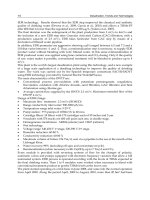
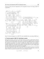
Figure 1 illustrates the modelled superstructure. All the possible alternative configurations and
interconnections between the three systems are embedded. The seawater feed passes through

a Sea Water Intake and Pre-treatment system (SWIP) where is chemically treated, according to
MSF and RO requirements. As Figure 1 shows, the feed stream of each process is not restricted
to seawater; instead, different streams can be blended to feed each system. Then, part of the
rejected stream leaving a system may enter into another one, even itself, resulting in a recycle.
The permeated streams of both RO systems and the distillate stream from MSF are blended to
produce the product stream, whose salinity is restricted to not exceed a maximum allowed salt
concentration. Furthermore, a maximum salt concentration is imposed for the blended stream
which is discharged back to the sea, in order to prevent negative ecological effects.


Fig. 1. Layout of the modelled superstructure
SWIP
Wfeed
msf
Wfeed
ro1
Wfeed
ro2
msf
F
W
ro2
F
W
MSF
HPP1
HPP2
RO1
RO2
msf

RM
W
ro1
Rro1
W
r
o
2
Rro2
W
msf
Rro2
W
msf
Rro1
W
msf
Rbdw
W
msf
P
W
ro1
Rro2
W
ro1
P
W
ro2
Rro1

W
ro2
P
W
ERS
ro1
Rbdw
W
ro2
Rbdw
W
ro1
RM
W
ro2
RM
W
PRODUCT
ro1
F
W
seawater
fresh water
brine
recycle
blow down
Optimization of Hybrid Desalination Processes
Including Multi Stage Flash and Reverse Osmosis Systems

313

Seawater characteristics: salt concentration and temperature are given data, as well as the
demand to be satisfied: total production and its maximum allowed salt concentration. On the
contrary, the flow rate of the seawater streams fed to each system are optimization variables,
as well as the flow rate and salt concentration of the product, blow down and inner streams.
The operating pressures for each RO system are also optimization variables. If the pressure
of the stream entering to a RO system is high enough, the corresponding high pressure
pumps are eliminated. Moreover, the number of modules operating in parallel at each RO
system is also determined by the optimization procedure. The remainder rejected flow rate
of both RO systems, if they do exist, will pass through an energy recovery system, before
being discharged back to the sea or fed into the MSF system.
For the MSF system, the geometrical design of the evaporator, the number of tubes in the
pre-heater, the number of flash stages, and others are considered as optimization variables.
The complete mathematical model is composed by four major parts: The Multi Stage Flash
model, The Reverse Osmosis model, network equations and cost equations. The following
section focuses on each of these four parts of the model.
3. Mathematical model
3.1 Multi Stage Flash model
The model representing the MSF system is based on the work (Mussati et al., 2004). A brief
description of the model is presented here.
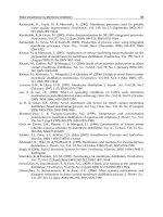
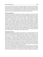
The evaporator is divided into stages. Each stage has a seawater pheheater, a brine flashing
chamber, a demister and a distillate collector. Figure 2 shows a flashing stage.


Fig. 2. Scheme of flashing stage
In a MSF system, feed stream passes through heating stages and is heated further in the heat
recovery sections of each subsequent stage. Then, feed is heated even more using externally
suplied steam. After that, the feedwater passes through various stages where flashing takes
place. The vapor pressure at each stage is controlled in such way that the heated brine enters
each chamber at the proper temperature and pressure to cause flahs operation. The flash
vapor is drawn to the cooler tube bundle surfaces where it is condensed and collected as

distillate and paseses on from stage to stage parallelly to the brine. The distillate stream is
also flash-boiled, so it can be cooled and the surplus heat recovered for preheating the feed.
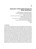
Figure 3 shows an scheme of a MSF system with NS stages.
Often, part of the brine leaving the last stage is mixed with the incoming feedwater because
it reduces the chemical pre-treatment cost. According to the interconections and
recirculations considered in the modeled superstructure, two typical MSF operating modes
are included: MSF-OT (without recycle) and MSF-BR (with recycle). However, more
complex configurations are also included, since different streams can be blended (at
different proportions) to feed the MSF system.
Brin
e
Brine flow
Demiste
r
Distillate tray
Tube bandle
Desalination, Trends and Technologies

314

12 3 NS-1 NS
F
msf
W
P
msf
W
R
msf
W

Q
D
es


Fig. 3. MFS system
The MSF model considers all the most important aspects of the process.
The heat consumption is calculated by:

F-6b
msf msf
10
Des
QWCpt
ρ
=Δ
(1)

= +
fe
tt tBPE
Δ
ΔΔ+ (2)
Total heat transfer area and number of flash stages are calculated as:

F
max msf
()/
F3
msf msf

10
= ln
f
TtT t
t
e
WCp
t BPE
A
Ut
−
Δ− Δ
⎛⎞
Δ−
⎜⎟
⎜⎟
Δ
⎝⎠
(3)

(
)
F
max msf
f
NS T t T t
=
−Δ − Δ (4)
The total production of distillate is evaluated by:

msf
PF
msf msf
11
NS
f
Cp t
WW
λ
⎡
⎤
Δ
⎛⎞
⎢
⎥
=−−
⎜⎟
⎜⎟
⎢
⎥
⎝⎠
⎣
⎦
(5)
The following equation establishes a relation between heat transfer area, number of tubes
and chamber width:

msf
π
tt

A
TD B N NS=
(6)
The stage height can be approximated by:
2
Hs Lb Ds
=
+ (7)
The number of rows of tubes in the vertical direction is related to the number of tubes in the
following way:

0.481
rt t
NTDN=
(8)
The following equation relates the shell diameter to the number of rows of tubes and Pitch:

2
rt t
Ds N P= (9)
Optimization of Hybrid Desalination Processes
Including Multi Stage Flash and Reverse Osmosis Systems

315
The length of the desaltor is constrained by the following two equations:

P-3
msf
msf
10

d
va
p
va
p
W
L
BV
ρ
= (10)

d
LDsNS=
(11)
The total stage surface area is calculated by:

msf msf
2 2
Sd d
ALB HsLHsBNS
=
++ (12)
Finally, the temperature of last flashing stage of the MSF system is calculated as:

RF
msf max msf

f
TT NStT t
=

−Δ= +Δ (13)
Despite the simplifying hypothesis assumed in the model, the MSF process is well
represented and the solutions of this model are accurately enough to establish conclusions
for the hybrid plant.
3.2 Reverse osmosis model
The model representing the RO system is based on the work (Marcovecchio et al., 2005). A
brief description of the equations is presented here.
Each RO system is composed by permeators operating in parallel mode and under identical
conditions. Particularly, data for DuPont B10 hollow fiber modules were adopted here.
However, the model represents the permeation process for general hollow fiber modules
and any other permeator could be considered providen the particular module parameters.
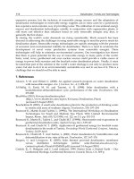
Figure 4 represents the RO system modeled for the hybrid plant.


Fig. 4. RO system
Initially, pressure of inlet stream is raised by the High Pressure Pumps (HPP). Then, the
pressurized stream passes through membrane modules, where permeation takes place. Part
of the rejected stream could pass through the energy recovery system, before being
discharged back to the sea or fed into the MSF system. Therefore, part of the power required
for the whole plant is supplied by the energy recovery system, and the rest will be provided
by an external source.
Equations (14) to (30) describe the permeation process taking place at one module of each
system.
HPP
ERS
F
ro
W
P
ro

W
R
ro
W
RO Permeators
Desalination, Trends and Technologies

316
The transport phenomena of solute and water through the membrane are modeled by the
Kimura-Sourirajan model (Kimura & Sourirajan, 1967):

(
)
bm P
bp
sss
w
ss
s
6
3600
10 101325
iRT ρ CC
J A PP
Ms
⎛⎞
−
⎜⎟
=−−
⎜⎟

⎜⎟
⎝⎠
s=ro1, ro2 (14)

(
)
mPb
ss
S
s
6
3600
10
BC C
ρ
J
−
= s=ro1, ro2 (15)
The velocity of flow is:

(
)
wS
ss
w
s
p
JJ
V
ρ

+
=
s=ro1, ro2 (16)
The following equation gives the salt concentration of the permeate stream:

S6
P
s
s
p
W
s
10J
C
V
ρ
= s=ro1, ro2 (17)
Permeate flow rate is calculated as the product between the permeation velocity and the
membrane area:

p
w
ssm
QVA= s=ro1, ro2 (18)
The total material balance for each permeator is:

p
fb
sss
QQQ=+ s=ro1, ro2 (19)

The salt balance in each permeator is given by:

p
fF bR P
ss s s s s
QC Q C Q C=+ s=ro1, ro2 (20)
The phenomenon of concentration polarization must be considered. The principal negative
consequence of this phenomenon is a reduction in the fresh water flow. The approach
widely used to model the influence of the concentration polarization is the film theory. The
Sherwood, Reynolds and Schmidt numbers are combined in an empirical relation: equation
(24) to calculate the mass transfer coefficient:

s0
s
2k r
Sh
D
=
s=ro1, ro2 (21)

Sb
0s
s
b
2
Re
rU
ρ
μ
= s=ro1, ro2 (22)

b
s
b
μ
Sc
ρ
D
= s=ro1, ro2 (23)
Optimization of Hybrid Desalination Processes
Including Multi Stage Flash and Reverse Osmosis Systems

317

()()
1/3 1/3
sss
2 725 Re Sh . Sc=
s=ro1, ro2 (24)
The concentration polarization phenomenon is modeled by:

mP w
ss s
RP
s
ss
exp
3600
CC V
k

CC
⎛⎞
−
=
⎜⎟
⎜⎟
−
⎝⎠
s=ro1, ro2 (25)
In order to estimate the average pressure drop in the fiber bore and the average pressure
drop on the shell side of the fiber bundle, it is necessary to calculate the superficial velocity
in the radial direction. According to (Al-Bastaki & Abbas, 1999), the superficial velocity can
be approximated as the log mean average of the superficial velocity at the inner and outer
radius of the fiber bundle:

f
si
s
s
i
3600 2 π
Q
U
RL
=
s=ro1, ro2 (26)

fw
so
ssm

s
o
3600 2 π
QVA
U
RL
−
=
s=ro1, ro2 (27)

()
si so
S
ss
s
si so
ss
log
UU
U
UU
−
= s=ro1, ro2 (28)
The approximation for the pressure drop in the fiber bore is based on Hagen-Poiseuille’s
equation:

p
w2
p
os

s
4
i
16
1
1
2
3600 101325
μ
rV L
P
r
=+ s=ro1, ro2 (29)
Similarly, the pressure drop on the shell side of the fiber bundle is estimated by Ergun’s
equation:

()
()
()
(
)
()
2
bS
2
bS
b
s
s
f

s
soi oi
32 3
pp
1.75 1
150 1
11
22
101325 101325
ερ U
εμU
P P RR RR
ε d ε d
−
−
=− − − − s=ro1, ro2 (30)
Finally, the total flow rates of feed and permeate for each system are given by:

Ff
sss
WNMQ= s=ro1, ro2 (31)

p
P
ss
s
WNMQ= s=ro1, ro2 (32)

The chosen model considers all the most important aspects affecting the permeation process.
Even thought, differential equations involved in the modeling are estimated without any

discretization, the whole model is able to predict the flow of fresh water and salt trough the
membrane in an accuracy way.
Desalination, Trends and Technologies

318
3.3 Network equations
The overall superstructure is modelled in such way that all the interconnections between the
three systems are allowed, as it shown in Figure 1.
In effect, part of the rejected stream of each system can enter into another system, even itself.
The fractions of rejected streams of RO systems that will enter into MSF system or that will
be discharged back to the sea, will pass through the ERS. On the contrary, the fractions of
rejected streams of RO systems that will enter into a RO system again, will not pass through
the ERS, because the plant could benefit from these high pressurized streams. In fact, when
all the streams entering to a RO system flow at a high enough pressure, the corresponding
HPPs can be avoided. That RO system would correspond to a second stage of reverse
osmosis. In that case, the pressure of all the inlet streams will be levelled to the lowest one,
by using appropriated valves. However, if at least one of the RO inlet streams is coming
from MSF system or from sea, the pressure of all the inlet streams will be lowered to
atmospheric pressure, and before entering membrane modules, HPPs will be required. The
network and cost equations are formulated is such way that the optimization procedure can
decide the existence or not of HPPs and this decision is correctly reflected in the cost functions.
When the whole model is optimized, the absence of a particular stream is indicated by the
corresponding flow rate being zero. Furthermore, the optimization procedure could decide
the complete elimination of one system for the optimal design. The energy and material
balances guarantee the correct definition of each stream.
The total fresh water demand is 2000 m
3
/h and is the result of blending the product stream
of each system:

PPP
msf ro1 ro2
WWWprodc++=
(33)
The fresh water stream must not exceed a maximum allowed salt concentration. This
requirement is imposed by the following constraint, taking into account that distillate
stream is free of salt, but permeate RO streams are not.

(
)
pp
PP
max ro1 ro1 ro2 ro2
ro1 ro2
cNMQCNMQCprodc≥+ (34)
For ecological reasons, the salinity of the blended stream which is discharged back to the sea
must not be excessively high. An acceptable maximum value for this salinity is 67000 ppm:

(
)
R Rbdw R Rbdw R Rbdw Rbdw Rbdw Rbdw
msf msf ro1 ro1 ro2 ro2 msf ro1 ro2
67000CWCWCW WWW++≤ ++ (35)
By considering all the possible streams that can feed MSF system, the following equations
give the flow rate of MSF feed stream:

FRMRMRM
msf msf msf ro1 ro2
WWfeedWWW= +++
(36)

Consequently, salt and energy balances for MSF feed are:

FF RRMRRMRRM
msf msf msf msf msf ro1 ro1 ro2 ro2
C W Cfeed Wfeed C W C W C W=+++ (37)

FF RRM RM RM
msf msf msf msf msf ro1 ro1 ro2 ro2
T W Tfeed Wfeed T W T W T W=+++ (38)
Optimization of Hybrid Desalination Processes
Including Multi Stage Flash and Reverse Osmosis Systems

319
The overall mass and salt balances for MSF system are given by:

F P RM Rro1 Rro2 Rbdw
msf msf msf msf msf msf
WWWW W W=++ + + (39)

(
)
FF R RM Rro1 Rro2 Rbdw
msf msf msf msf msf msf msf
CW C W W W W=+++ (40)
Similarly to equation (36), the following equations give the flow rate of RO feed streams:

F Rro1 Rro1 Rro1
ro1 ro1 msf ro1 ro2
WWfeedWWW= +++ (41)

F Rro2Rro2Rro2
ro2 ro2 msf ro1 ro2
WWfeedW W W= +++ (42)
Equations (43) and (44) establish the division of the total rejected stream leaving each RO
system in the different assignations:

bRMRro1Rro2Rbdw
ro1 ro1 ro1 ro1 ro1 ro1
NM Q W W W W=+ + +
(43)

bRMRro1Rro2Rbdw
ro2 ro2 ro2 ro2 ro2 ro2
NM Q W W W W=+ + + (44)
The salt balances for RO system feeds are:

F F R Rro1 R Rro1 R Rro1
ro1 ro1 ro1 msf msf ro1 ro1 ro2 ro2
CW CfeedWfeed C W CW CW=+++ (45)

F F R Rro2 R Rro2 R Rro2
ro2 ro2 ro2 msf msf ro1 ro1 ro2 ro2
C W Cfeed Wfeed C W C W C W=+++ (46)
Meanwhile, energy balances for RO systems feeds are given by:

F R Rro1 Rro1 Rro1
ro1 ro1 ro1 msf msf ro1 ro1 ro2 ro2
T W Tfeed Wfeed T W T W T W=+++ (47)

F R Rro2 Rro2 Rro2

ro2 ro2 ro2 msf msf ro1 ro1 ro2 ro2
T W Tfeed Wfeed T W T W T W=+++ (48)
The overall mass balances for RO systems are:

F P RM Rro1 Rro2 Rbdw
ro1 ro1 ro1 ro1 ro1 ro1
WWW W W W=+ + + + (49)

F P RM Rro1 Rro2 Rbdw
ro2 ro2 ro2 ro2 ro2 ro2
WWW W W W=+ + + +
(50)
The following equations establish the overall salt balances for RO systems:

(
)
F F P P R RM Rro1 Rro2 Rbdw
ro1 ro1 ro1 ro1 ro1 ro1 ro1 ro1 ro1
CW CW C W W W W=+ +++ (51)

(
)
FF PP R RM Rro1 Rro2 Rbdw
ro2 ro2 ro2 ro2 ro2 ro2 ro2 ro2 ro2
CW CW C W W W W=+ +++ (52)
Equations (53) to (60) assign to the variables P
ro1
in
and P
ro2

in
the minimal pressure over all
the flows entering to the corresponding RO system. This assignation will allow the model to
decide whether the HPPs before each RO system are necessary or not. In fact, if the minimal
Desalination, Trends and Technologies

320
pressure of the inlet streams: P
in
is equal or greater than the pressure needed to pass
through the membrane modules: P
f
, then the corresponding HPPs are not necessary. On the
other hand, if the value of P
in
does not reach the operating pressure P
f
, then the
corresponding HPPs cannot be avoided. In the following section, this decision will be
modelled by the cost functions.
If the stream feeding the RO1 system includes part of brine stream leaving the MSF system,
equation (53) imposes that the corresponding variable P
ro1
in
be lower or equal than
atmospheric pressure. On the contrary, if no stream coming from MSF system is feeding the
RO1 system (i.e. W
msf
Rro1
=0), then constraint (53) does not affect variable P

ro1
in
at all.
Equation (56) performs the same imposition by evaluating the existence or not of stream
coming from the sea in the RO1 feed.
Equations (54) and (55) evaluate the existence of streams coming from an RO system and
feeding RO1 system. If any of these streams does exist (i.e. W
ro1
Rro1
>0 or W
ro2
Rro1
>0), the
variable P
ro1
in
is imposed to be lower than the pressure of the corresponding stream.

(
)
Rro1 in
msf ro1
10WP
−
≤ (53)

(
)
Rro1 in b f
ro1 ro1 ro1 ro1

(2 ) 0WP PP
−
−≤ (54)

(
)
Rro1 in b f
ro2 ro1 ro2 ro2
(2 ) 0WP PP
−
−≤ (55)

(
)
in
ro1 ro1
10Wfeed P
−
≤ (56)
Equations (57) to (60) act in analogous way to the four previous ones for the system RO2.

(
)
Rro2 in
msf ro2
10WP
−
≤
(57)

(
)
Rro2 in b f
ro1 ro2 ro1 ro1
(2 ) 0WP PP
−
−≤ (58)

(
)
Rro2 in b f
ro2 ro2 ro2 ro2
(2 ) 0WP PP
−
−≤ (59)

(
)
in
ro2 ro2
10Wfeed P
−
≤ (60)
When the HPPs before an RO system are avoided, it is not convenient that the
corresponding system operates at pressure lower than the available one. The following
equations guarantee that, and also ensure the correct definition of associated cost functions.

fin
ro1 ro1
PP≥ (61)

fin
ro2 ro2
PP≥ (62)
Most of the constraints presented in this section are complementary to the cost functions
described in the following section.
Optimization of Hybrid Desalination Processes
Including Multi Stage Flash and Reverse Osmosis Systems

321
3.4 Cost equations
This section describes the cost equations of the total plant. The objective function to be
minimized is the cost per m
3
of produced fresh water. Capital and operating costs are
calculated. The cost equations were formulated in such way that they can correctly reflect
the presence or absence of equipments, streams or systems.
Capital costs are calculated by equations (63) to (67), while equations (69) to (76) estimate
the operating ones.
Cost function reported by (Malek et al., 1996) was adopted in order to estimate capital cost
for the SWIP:

()
0.8
swip msf ro1 ro2
996 ( ) 24cc Wfeed Wfeed Wfeed=++ (63)
Capital cost of HPP is defined in the same way. As it was explained at section 3.3, the
variables P
in
assume the minimal pressure over all the streams feeding a RO system, while

P
f
is the operating pressure of the system. Equations (64) and (65) along with the
optimization procedure, will make the variables cc
hpp
to assume the capital cost of the HPP
only when P
f
> P
in
, otherwise cc
hpp
will assume value null.

()()
F
ffin
ro1
hpp1 ro1 ro1 ro1
393000 10710 1.01325 0
450
W
cc P P P
⎛⎞
−
+⋅−≥
⎜⎟
⎜⎟
⎝⎠
(64)

()()
F
ffin
ro2
hpp2 ro2 ro2 ro2
393000 10710 1.01325 0
450
W
cc P P P
⎛⎞
−
+⋅−≥
⎜⎟
⎜⎟
⎝⎠
(65)
Capital cost of the ERS is similar to the HPP one, since it consists of a reverse running
centrifugal pump. Taking into account flow rate and pressure of the streams passing
through the ERS, the capital cost is given by:

()
()
Rbdw RM
bf
ro1 ro1
ers ro1 ro1
Rbdw RM
bf
ro2 ro2

ro2 ro2
()
393000 10710 (2 - ) 1.01325
450
()
393000 10710 (2 - ) 1.01325
450
WW
cc P P
WW
PP
+
=
++
+
+
(66)
The capital cost considered for the MSF system is the one due to the heat transfer area.
According to (Mussati et al., 2006) this cost can be estimated as:
cc
area
= (A
t
+ A
S
25) 50 (67)
Therefore, the plant equipment cost is: cc
eq
= cc
swip

+ cc
hpp1
+ cc
hpp2
+ cc
area
. Civil work cost is
estimated as a 10% of cc
eq
(Wade, 2001). Indirect cost is estimated in the same way (Helal et
al., 2003). Then, the Total Capital Cost (TCC) is given by:
TCC = cc
eq
+ cc
cw
+ cc
i
= 1.2 cc
eq
= 1.2 (cc
swip
+ cc
hpp1
+ cc
hpp2
+ cc
ers
+ cc
area
) (68)

Capital charge cost is estimated as a 8% of the total capital cost (Malek et al., 1996):
co
c
= 0.08 TCC (69)
Desalination, Trends and Technologies

322
The cost due to permeators is included as operative cost, by calculating their annualized
installation cost and considering the replacement of 20% of permeators per year. According
to (Wade, 2001) this sum can be estimated as $397.65 per module per year.
co
rp
= (NM
ro1
+ NM
ro2
) 397.65 (70)
Energy cost is calculated by using the cost function given in (Malek et al., 1996) and the
power cost reported in (Wade, 2001). The energy required by the SWIP and the HPP; and
the energy provided by the ERS must be taken into account:

swip msf ro1 ro2
ec
swip
() 24
=0.03
P Wfeed Wfeed Wfeed
co f
eff
⎛

++
⎜
⎜
⎝

fin F fin F
ro1 ro1 ro1 ro2 ro2 ro2
hpp hpp
( - ) 1.01325 24 ( - ) 1.01325 24PP W PP W
eff eff
++

b f Rbdw RM b f Rbdw RM
ers ro1 ro1 ro1 ro1 ers ro2 ro2 ro2 ro2
1.01325 (2 - ) 24 ( ) 1.01325 (2 - ) 24 ( )eff P P W W eff P P W W
⎞
−+− +
⎟
⎟
⎠

(71)

Spares costs are calculated by using the estimated values reported by (Wade, 2001):

PP P
sro1ro2c msfc
= 24 365 ( ) 0.033 + 24 365 0.082co W W f W f+
(72)
Chemical treatment costs is calculated using the cost per m

3
of feed reported in (Helal et al.,
2003):

Rro1 Rro2
ch ro1 msf ro2 msf c
24 365 ( ) 0.018co Wfeed W Wfeed W f=+++

RM RM
msf ro1 ro2 c
24 365 ( ) 0.024Wfeed W W f+++

(73)

General operation and maintenance cost is calculated according to the value per m
3
of
produced water reported in (Wade, 2001):

PPP
om msf ro1 ro2 c
= 24 365 ( ) 0.126co W W W f++ (74)
Similarly, power cost for MSF system is evaluated according to (Wade, 2001):

P
pw msf c
= 24 365 0.109co W f (75)
The cost of the heat consumed by MSF system is calculated by using the function proposed
by (Helal et al., 2003):
co

ht
= 24 365 f
c
(Q
Des
10
6
/
λ
) (T
max
-323) 0.00415 /85 (76)
Finally, the Annual Operating Cost (AOC) is given by:
AOC = co
c
+co
rp
+co
e
+co
s
+co
ch
+co
om
+co
pw
+co
ht
(77)

By considering a plant life of 25 years (n) and a discount rate of 8% (i), capital recovery
factor can be calculated, giving: crf=((i+1)
n
-1)/(i(i+1)
n
). Finally, fresh water cost per m
3
is
given by:
Optimization of Hybrid Desalination Processes
Including Multi Stage Flash and Reverse Osmosis Systems

323
cos
24 365
TCC cr
f
AOC
t
prodc
+
= (78)
Equations (1) to (78) define the model for the design and operation of a hybrid desalination
plant, including MSF and RO systems.
In the following section, this model will be optimized for different seawater salt
concentrations, and the obtained solutions will be analysed.
4. Results: Optimal plant designs and operating conditions
In this section optimized results are presented and discussed.
The proposed optimization problem P is defined as follows:

P: minimize cost
s. t. Equations (1) to (78)
while all the variables have appropriated bounds.
The optimization procedure will look for the optimal layout and operating conditions in
order to minimize the cost per m
3
of produced fresh water.
It is important to note that almost all discrete decisions were modelled exploiting the actual
value of flow rates and pressures. Thus, no binary decision variables were included into the
model. Only four integer variables are involved: the number of flash stages and the number
of tubes in the pre-heater at the MSF system; and the number of permeators operating in
parallel at each RO system.
Tables 1 and 2 list the parameter values used for the RO and MSF systems, respectively.

Parameters for RO systems
i, number of ions for ionized solutes 2
R, ideal gas constant, N m / kgmole K 8315
Ms, solute molecular weight 58.8
T, seawater temperature, ºC 25
ρ
b
, brine density, kg/m
3
1060
ρ
p
, pure water density, kg/m
3

1000

μ
p
, permeated stream viscosity, kg/m s
0.9x10
-3

μ
b
, brine viscosity, kg/m s

1.09x10
-3

D, diffusivity coefficient, m
2
/s

1x10
-9

P
swip
, SWIP outled pressure, bar

5
eff
swip
, intake pump efficiency

0.74

eff
hpp
, high pressure pumps efficiency

0.74
eff
ers
, energy recovery system efficiency

0.80
f
c
, load factor

0.90
Table 1. Parameters for RO systems
Desalination, Trends and Technologies

324
Parameters and operating ranges of the particular hollow fiber permeator were taken from
(Al-Bastaki &Abbas, 1999; Voros et al., 1997). These specifications constitute constants and
bounds for some variables of the model.

Parameters for MSF system
T
max
, K 385
Cp
msf
, Kcal/(kg K) 1

TD, m 0.030
Pitch: P
t
1.15
BPE, K 1.9
U, Kcal/m
2
/K/h 2000
λ
, Kcal/Kg
550
Table 2. Parameters for MSF system
The optimization model was implemented in General Algebraic Modeling System: GAMS
(Brooke et al., 1997) at a Pentium 4 of 3.00 GHz. At first, the MINLP solver DICOPT was
implemented to solve the problem. Unfortunately, the solver failed to find even a feasible
solution for most case studies. Then, other resolution strategy was carried out in order to
tackle the problem and obtain the optimal solutions.
Since it involves only 4 integer variables, the problem was solved in 2 steps. Firstly, the
relaxed NLP problem was solved, i.e., the integer variables were relaxed to continuous ones.
Departing from the optimal solution of the relaxed problem, the MINLP was solved by
fixing the integer variables at the nearest integer values and optimizing the remaining
variables. Since the MINLP problem presents a lot of non-convexities, a global search
strategy was also implemented. In fact, for each study case, the previous 2 steps were
repeated starting the optimization search from different initial points, and then, the best
local optimal solution was selected. The generalized reduced gradient algorithm CONOPT
was used as NLP solver. This resolution procedure was successful, providing optimal
solutions in all case studies. The total CPU time required to solve all the cases was 1.87s,
what proves that the proposed procedure is highly efficient and the model is
mathematically good conditioned.
11 case studies were solved for seawater salt concentration going from 35000 ppm up to

45000 ppm. The total production was fixed at 2000m
3
/h with a maximum allowed salt
concentration of 570 ppm.
Table 3 shows the values of the main interconnection variables for the optimal solutions:
feed flow rates, product and internal streams, as well as their salt concentrations.
Table 4 reports design variables and operating conditions for each process for the optimal
solutions.
For seawater salt concentrations between 35000 and 38000 ppm, the optimal solutions do not
include the MSF system. In fact, for these salinities, the optimal hybrid plant designs consist
on a typical two stage RO plant. However, if the seawater salinity is greater than 38000 ppm,
both desalination processes are present in the optimal design of the plant; that is: including
MSF system is profitable.
Figure 5 shows a scheme of the optimal design of the plant obtained for seawater salinities
between 35000 and 38000 ppm.
Optimization of Hybrid Desalination Processes
Including Multi Stage Flash and Reverse Osmosis Systems

325


45000
561.9
1438.1
1947.5
4091.6
-
4546.9
561.9
2599.4

-
-
1385.6
4091.6
1044.6
-
-
3047.2
-
3047.2
393.7
-
-
-
2653.4
55431.6
63247.0
45000
592.1
60220.3
60220.3
1324.8
68959.8
0.9198
44000
496.4
1503.6
1631.7
4144.8
-

4073.0
496.4
2441.3
-
-
1135.3
4144.8
1095.8
-
-
3049.0
-
3049.0
407.8
-
-
-
2641.2
55530.6
63237.4
44000
566.1
59610.0
59610.0
1274.4
68617.4
0.8968
43000
428.8
1571.2

1336.0
4199.9
-
3574.3
428.8
2238.3
-
-
907.2
4199.9
1149.1
-
-
3050.8
-
3050.8
422.1
-
-
-
2628.6
55726.6
63322.7
43000
541.5
58992.1
58992.1
1226.4
68269.1
0.8726

42000
358.5
1641.5
1057.7
4256.7
-
3044.2
358.5
1986.5
-
-
699.2
4256.7
1204.8
-
-
3051.8
-
3051.8
436.8
-
-
-
2615.0
56050.2
63531.0
42000
518.2
58375.5
58375.5

1180.6
67928.1
0.8486
41000
285.9
1714.1
794.6
4315.4
-
2444.1
285.9
1599.3
-
-
558.8
4315.4
1262.4
-
-
3053.0
-
3053.0
451.7
50.2
-
-
2551.2
56833.3
64363.0
41000

496.2
57747.9
57747.9
1137.1
67577.7
0.8240
40000
210.6
1789.4
543.9
4376.8
-
1808.6
210.6
1169.2
-
-
428.7
4376.8
1322.5
-
-
3054.3
-
3054.3
466.9
95.4
-
-
2492.0

58059.1
65712.0
40000
475.3
57113.9
57113.9
1095.3
67221.6
0.7985
39000
132.4
1867.6
304.0
4441.0
-
1146.4
132.4
725.4
-
-
288.6
4441.0
1385.2
-
-
3055.8
-
3055.8
482.4
117.1

-
-
2456.3
60317.6
68194.8
39000
455.4
56472.6
56472.6
1055.3
66861.1
0.7717
38000
-
2000
-
4790.1
-
-
-
-
-
-
-
4790.1
1540.7
-
-
2808.8
440.6

2808.8
459.3
-
-
-
2349.5
-
-
38000
437.8
55810.8
55810.8
1013.6
66522.5
0.7410
37000
-
2000
-
4498.0
-
-
-
-
-
-
-
4498.0
1492.3
-

-
3005.7
-
3005.7
507.7
-
-
-
2498.0
-
-
37000
419.8
55160.9
55160.9
978.9
66174.0
0.7121
36000
-
2000
-
4373.0
-
-
-
-
-
-
-

4373.0
1495.1
-
-
2877.9
-
2877.9
504.9
-
-
-
2373.0
-
-
36000
402.4
54493.6
54493.6
951.6
65884.8
0.6952
35000
-
2000
-
4241.3
-
-
-
-

-
-
-
4241.3
1499.6
-
-
2741.7
-
2741.7
500.4
-
-
-
2241.3
-
-
35000
383.8
53934.2
53934.2
940.5
65764.6
0.6784
F
P
RM
Rro1
Rro2
Rbdw

F
P
RM
Rro1
Rro2
Rbdw
F
P
RM
Rro1
Rro2
Rbdw
F
R
F
P
R
F
P
R
Optimal solutions for the hybrid plant: MSF-RO. Total Production: 2000m
3
/h. Maximum allowed salt concentration: 570pm
Seawater salinity Cfeed,
ppm

Production flow rates for MSF and RO processes
W
msf
P

, m
3
/h
(W
ro1
P
+ W
ro2
P
), m
3
/h
Seawater feed: Wfeed, m
3
/h
MSF
RO1
RO2
Flow rates of the interconnection streams: W, m
3
/h
MSF
MSF
MSF
MSF
MSF
MSF
RO1
RO1
RO1

RO1
RO1
RO1
RO2
RO2
RO2
RO2
RO2
RO2
Salt concentration o
f the interconnection streams: C, ppm
MSF
MSF
RO1
RO1
RO1
RO2
RO2
RO2
Cost of fresh water, $/m
3

Table 3. Optimal solutions for the hybrid plant: interconnection variables
Desalination, Trends and Technologies

326
Optimal solutions for the hybrid plant: MSF-RO. Design variables and operating conditions.
Seawater
salinity:
Cfeed, ppm

35000 36000 37000 38000 39000 40000 41000 42000 43000 44000 45000
MSF
Q
Des
,
Gcal/h
- - - - 8.80 12.93 16.78 20.46 23.89 27.10 30.14
NS
- - - - 19 23 26 28 30 32 33
A
S
, m
2
- - - - 828.8 1103.5 1332.8 1515.5 1679.8 1836.0 1957.8
A
t
, m
2
- - - - 11858.919552.9 27100.3 34308.4 40568.8 46406.2 52594.8
Δt, K
- - - - 7.24 6.75 6.48 6.34 6.30 6.28 6.25
Δt
f
, K
- - - - 3.54 2.95 2.63 2.46 2.34 2.23 2.19
Δt
e
, K
- - - - 1.80 1.89 1.95 1.99 2.07 2.15 2.16
N

t

- - - - 368 501 615 723 798 855 940
L
d
, m - - - - 8.55 12.09 15.13 17.66 19.88 21.96 23.74
Hs, m - - - - 1.45 1.53 1.58 1.63 1.66 1.67 1.72
D
S
, m - - - - 0.45 0.53 0.58 0.63 0.66 0.67 0.72
T
msf
F
, K - - - - 310.5 310.3 310.3 309.9 308.6 307.4 306.3
T
msf
R
, K - - - - 317.7 317.1 316.7 316.2 314.9 313.7 312.6
RO1
NM
1
4633 4777 4915 5232 4843 4773 4706 4642 4580 4520 4462
P
f
1
, atm 67.900 67.900 67.900 67.899 67.900 67.900 67.899 67.900 67.893 67.898 67.900
HPP1 yes yes yes yes yes yes yes yes yes yes yes
T
ro1
, K

298.0 298.0 298.0 298.0 298.0 298.0 298.0 298.0 298.0 298.0 298.0
RO2
NM
2
3129 3189 3286 3063 3332 3331 3330 3328 3327 3325 3323
P
f
2
, atm 67.868 67.868 67.868 67.866 67.867 67.867 67.867 67.867 67.860 67.865 67.866
HPP2 no no no no no no no no no no no
T
ro2
, K 298.0 298.0 298.0 298.0 298.0 298.0 298.0 298.0 298.0 298.0 298.0
Table 4. Optimal solutions for the hybrid plant: design variables and operating conditions


Fig. 5. Scheme of the optimal design for seawater salinities between 35000 and 38000 ppm
The stream with flow rate W
ro1
Rbdw
is only present for 38000 ppm of seawater salinity. For
salinities lower than 38000 ppm, the totality of the stream rejected from the first RO stage:
system RO1, enters into the second RO stage: system RO2. Then, the stream entering into
the system RO2 is sufficiently pressurized. Therefore, the high pressure pumps before
system RO2 are avoided in the optimal solutions. This decision is properly made by the
optimization procedure, and it is correctly reflected in the cost function.
RO2
SWIP
Wfeed

ro1
ro2
F
W
ro1
F
W
RO1
ro2
P
W
ro1
Rro2
W
ro1
P
W
ERS
ro2
Rbdw
W
ro1
Rbdw
W
PRODUCT
HPP1
Optimization of Hybrid Desalination Processes
Including Multi Stage Flash and Reverse Osmosis Systems

327

Figure 6 shows a scheme of the optimal solutions obtained for seawater salt concentrations
between 39000 and 45000 ppm.
For these case studies, both desalination processes are present at the optimal hybrid plant
design. The RO systems work as a two-stage RO plant, i.e.: system RO1 is fed directly from
sea, while its rejected stream is the fed stream for system RO2. No other streams are blended
to feed RO systems.
Regarding MSF system, it operates with an important recycle. This re-circulated stream
reduces the chemical pre-treatment and raises the feed stream temperature with the
consequent reduction of external heat consumption. Both factors straightly impact on the
final cost.


Fig. 6. Scheme of the optimal design for seawater salinities between 39000 and 45000 ppm
As it is also shown in Table 3, the three first cases presented in Figure 6 include the stream
with flow rate W
ro2
RM
. However, for seawater salt concentrations higher than 41000 ppm this
flow rate is null and the stream does not exist. Then, for the last four case studies, even
though the two desalination processes are selected for the optimal plant design, they operate
in independent way. In fact: there is no stream connecting the MSF and RO processes.
However, both processes share the intake and pre-treatment system. Furthermore, the
salinity of the product stream satisfies the maximum allowed salt concentration requirement
because the three product streams are blended. As it can be seen at Table 3, if only the
permeate streams coming from RO systems are blended, then the salt concentration of the
resulting stream will be far above the maximum allowed salt concentration.
Again, the stream feeding system RO2 is composed only by the stream rejected from system
RO1 and it is high pressurized. Thus, the high pressure pumps before system RO2 are
unnecessary and consequently, they are avoided at the optimal design.
Figure 7 shows the fresh water produced by each desalination process for all the case

studies.
As it was mentioned, for seawater salt concentrations below 38000 ppm, MSF system is not
present, thus the demand is totally satisfied by RO systems. On the other hand, for seawater
salinities higher than 38000 ppm, both processes contribute to satisfy the demand. Although
the RO systems produce more fresh water than MSF system, the MSF production increases
according to the seawater salinity rise.
SWIP
Wfeed
msf
Wfeed
ro1
msf
F
W
ro2
F
W
ro1
F
W
MSF
HPP1
RO2
RO1
msf
RM
W
msf
Rbdw
W

msf
P
W
ro2
P
W
ro1
Rro2
W
ro1
P
W
ERS
ro2
Rbdw
W
ro2
RM
W
PRODUCT
Desalination, Trends and Technologies

328



Fig. 7. Fresh water production
If the MSF system would not be considered, for the optimal design of a two stage RO plant
the capacity of the second stage will decrease when the seawater salinity increases
(Marcovecchio et al., 2005). In fact, even though the stream rejected from the first RO stage is

high pressurized and it could enter into a second stage with no need of high pressure
pumps; in the optimal design, part of this stream is discharged back to the sea. The second
stage capacity will continue decreasing until only one RO stage is the optimal design for
high feed salt concentration. The reason why it is no longer profitable to use the stream
rejected from the first RO stage is that its salinity is too high. Thus, the salt concentration of
the potential permeate will be lower but also high and then, it is not possible to satisfy the
maximum allowed salt concentration even by blending with the first stage permeate.
Therefore, the fresh water produced by the first stage must be higher in order to satisfy the
demand. Consequently, the flow rate of seawater is increased. As a consequence, the cost
per m
3
of fresh water increases, since many costs are directly affected.
Contrary, in a hybrid plant where the MSF process is available, in that break point where the
optimal design of a RO plant changes, it begins to be profitable to complement the RO
production with distillated from MSF system.
Then, for feed salinities higher than 38000 ppm, the growth of MSF system production is
approximately linear. With this plant design, there is no stream rejected from the first RO
stage being discharged back to the sea, i.e. the totality of that stream enters into the second
RO stage. And the total production of the plant reaches the requirement of maximum
allowed salt concentration by blending the slightly concentrated permeate from RO systems
with the free of salt distillate of MSF process.
Finally, Figure 8 compares the cost per m
3
of fresh water produced with the optimal
configurations obtained for the hybrid plant with those obtained for the RO stand alone
plant.
As it is shown in Figure 8, the cost reduction reached with the hybrid RO-MSF plant is
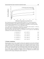
considerable. For feed salinities between 39000 and 44000 ppm, the cost function has an