Báo cáo toán học: "Bounds for the H¨ckel energy of a graph u" pptx
Bạn đang xem bản rút gọn của tài liệu. Xem và tải ngay bản đầy đủ của tài liệu tại đây (147.32 KB, 12 trang )
Bounds for the H¨uckel energy of a graph
Ebrahim Ghorbani
1,2,∗
, Jack H. Koolen
3,4,†
, Jae Young Yang
3,‡
e
1
Department of Mathematical Sciences, Sharif University of Technology,
P.O. Box 11155-9415 , Tehran, Iran
2
School of Mathematics, Institute for Research in Fundamental Sciences (IPM),
P.O. Box 19395-5746 , Tehran, Iran
3
Department of Mathematics, POSTECH, Pohang 790-785, South Korea
4
Pohang Mathematics Institute, POSTECH, Pohang 790-785, South Korea
Submitted: Oct 9, 2009; Accepted: Oct 25, 2009; Published: Nov 7, 2009
Mathematics Subject Classifications: 05C 50, 05E30
Abstract
Let G be a graph on n vertices with r := ⌊n/2⌋ and let λ
1
··· λ
n
be
adjacency eigenvalues of G. Then the H¨uckel energy of G, HE(G), is defined as
HE(G) =
2
r
i=1
λ
i
, if n = 2r;
2
r
i=1
λ
i
+ λ
r+1
, if n = 2r + 1.
The concept of H¨uckel energy was introduced by Coulson as it gives a good ap-
proximation for the π-electron energy of molecular graphs. We obtain two upper
bounds and a lower bound for HE(G). When n is even, it is shown that equality
holds in both upper bounds if and only if G is a str ongly regular graph with pa-
rameters (n, k, λ, µ) = (4t
2
+ 4t + 2, 2t
2
+ 3t + 1, t
2
+ 2t, t
2
+ 2t + 1), for positive
integer t. Furthermore, we will give an infinite family of these strongly regular graph
whose construction was communicated by Willem Haemers to us. He attributes the
construction to J.J. Seidel.
∗
This work was done while the first author was visiting the department of mathematics of POSTECH.
He would like to thank the department for its hospitality and support.
†
JHK was partially supported by a grant from the Korea Research Foundation funded by the Korea n
government (MOEHRD) under grant number KRF-2007-412-J02302.
‡
The results in this paper were obtained as a part of an Undergraduate Research Project of POSTECH
under project number 2.0005656.01 and JYY greatly thanks POSTEC H for its support.
the electronic journal of combinatorics 16 (2009), #R134 1
1 Introduction
Throughout this paper, all graphs are simple and undirected. Let G be a graph with n
vertices and A be the adjacency matrix o f G. Then the eigenvalues of G are defined as the
eigenvalues of A. As all eigenvalues of A are real, we can rearra nge them as λ
1
··· λ
n
.
I. Gutman (see [9]) defined the energy of G, E(G), by
E(G) :=
n
i=1
|λ
i
|.
In chemistry, the energy of a given molecular graph is of interest since it can be related
to the tota l π-electron energy of the molecule represented by that graph. The reason for
Gutman’s definition is that E(G) gives a good approximation for the π-electron energy
of a molecule where G is then the corresponding molecular gra ph. For a survey on the
energy of graphs, see [9]. The H¨uckel energy of G, denoted by HE(G), is defined as
HE(G) =
2
r
i=1
λ
i
, if n = 2r;
2
r
i=1
λ
i
+ λ
r+1
, if n = 2r + 1 .
The idea of introducing H¨uckel energy (implicitly) exists in Erich H¨uckel’s first paper
[10] in 1931 and is also found in his book [11]. The concept was explicitly used in 1940
by Charles Coulson [2] but, most probably, can be found also in his earlier articles. In
a “canonical” fo r m, the theory behind the H¨uckel energy was formulated in a series of
papers by Coulson and Longuet-Higgins, of which the first (and most important) is [3].
In comparison with energy, the H¨uckel energy of a gra ph gives a better approximation
for the total π-electron energy of the molecule represented by that graph, see [7]. Clearly
for a graph G vertices, HE(G) E(G), and if G is bipartite, then equality holds. Koolen
and Moulton in [12, 13] gave upp er bounds on the energy of graphs and bipartite graphs,
respectively. These bounds have been generalized in several ways. Obviously, the upper
bounds of Koolen and Moulton also give upper bounds for the H¨uckel energ y of graphs.
In this paper, we obtain better upper bounds for the H¨uckel energy of a graph. More
precisely, we prove that for a graph G with n vertices and m edges,
HE(G)
2m
n−1
+
√
2m(n−2)(n
2
−n−2m)
n−1
, if m
n
3
2(n+2)
;
2
n
mn(n
2
− 2m) <
4m
n
, otherwise;
(1)
if n is even, and
HE(G)
2m
n−1
+
√
2mn(n
2
−3n+1)(n
2
−n−2m)
n(n−1)
if m
n
2
(n−3)
2
2(n
2
−4n+11)
;
1
n
2m(2n − 1)(n
2
− 2m), otherwise;
(2)
if n is o dd. Then we show that
HE(G)
n
2
1 +
√
n − 1
, (3)
the electronic journal of combinatorics 16 (2009), #R134 2
if n is even, and
HE(G) <
n
2
1 +
√
n −
1
√
n
, (4)
if n is odd. Moreover, equality is attained in (1) if and only if equality attained in (3) if
and only if G is a strongly regular graph with parameters (n, k, λ, µ) = (4t
2
+ 4t + 2, 2t
2
+
3t + 1, t
2
+ 2t, t
2
+ 2t + 1). The proofs of the above upper bounds are given in Section 2.
It is known that E(G) 2
√
n − 1 for any graph G on n vertices with no isolated vertices
with equality if and only if G is the star K
1,n−1
(see [4]). In Section 3, we prove that
the same bound holds for H¨uckel energy. In the last section, we give a construction of
srg(4t
2
+ 4t + 2, 2t
2
+ 3t + 1, t
2
+ 2t, t
2
+ 2t + 1).
2 The upper bound for H¨uckel energy
In this section we prove (1), (2), (3), and (4). The equality cases are also discussed. We
begin by stating a lemma which will be used later.
Lemma 1. Let G be a graph with n vertices and m edges. Suppose r := ⌊n/2⌋ and
α :=
r
i=1
λ
2
i
(G).
If m n − 1 2, then
α
r
4m
2
n
2
. (5)
Proof. First, suppose m n. Then G contains a cycle, and so by interlacing, we see
λ
2
n
+ λ
2
n−1
2. Therefore, α/r (2m −2)/r 4m
2
/n
2
. If m = n −1 and G is connected,
then G is a tree. Thus α = m, and obviously (5) holds. So in the rest of proof we assume
that G is disconnected and m = n − 1. If G has at least three non-trivial components,
then at least one of the components contains a cycle. The component containing a cycle
has either an eigenvalue at most −2, or two eigenvalues −1 and the other two
components have an eigenvalue −1. It turns out that λ
2
n
+ λ
2
n−1
+ λ
2
n−2
+ λ
2
n−3
4
where n 7. Hence
α 2m −4. (6)
It is easily seen that (5) fo llows from (6). Now, suppose that G has two non-trivial
connected components G
1
and G
2
, say. Let G
1
, G
2
have n
1
, n
2
vertices and m
1
, m
2
edges,
respectively. First suppose n
1
, n
2
3. If G
1
or G
2
contains a K
1,2
as an induced subgraph,
we are done by interlacing. So one may assume that both G
1
and G
2
contain a triangle.
It turns out that m
1
n
1
and m
2
n
2
. Hence G must have an isolated vertex which
implies n 7. On the other hand, by interlacing, the four smallest eigenvalues of G are
at most −1 implying (6). Now, assume that n
1
= 2. So G
2
must contain a cycle C
ℓ
. We
may assume that C
ℓ
has no chord. If ℓ 4, we are done. So let ℓ = 3. If n
2
= 3, then
G does not have isolated vertices, i.e., G = C
3
∪ K
2
, for which (5) holds. Thus n
2
4
the electronic journal of combinatorics 16 (2009), #R134 3
Figure 1: The paw and the diamond graphs
which means that at least one of the diamond graph, the paw graph (see Figure 1), or
K
4
is induced subgraph of G. If it contains either the diamond or the paw graph, we are
done by interlacing. If it contains K
4
, then G must have at least two isolated vertices, i.e.,
n 8. Thus the four smallest eigenvalues of G are at most −1 which implies (6). Finally,
assume that G has exactly one non-trivial component G
1
with n
1
vertices. It turns out
that n
1
3 and G
1
contains a cycle. By looking at the table o f graph spectra of [5, pp.
272–3], it is seen that if n
1
= 3, 4, G satisfies (5). If n
1
5, then making use of the
table mentioned above and interlacing it follows that λ
2
n
+ λ
2
n−1
+ λ
2
n−2
4 unless G
1
is a
complete graph in which case G has at least 11 vertices and the four smallest eigenvalues
of G is −1, implying the result. ✷
2.1 Even order graphs
In this subsection we prove (1) and (3) for graphs of an even order. The cases of equalities
are also characterized.
Theorem 2. Let G be a graph on n vertices and m edges where n is even. Then (1)
holds. Moreover, equality holds if and only if n = 4t
2
+ 4t + 2 for some positive integer
t, m = (2t
2
+ 2t + 1)(2t
2
+ 3t + 1) and G is a strongly regular graph with parameters
(n, k, λ, µ) = (4t
2
+ 4t + 2, 2t
2
+ 3t + 1, t
2
+ 2t, t
2
+ 2t + 1).
Proof. Let n = 2r and λ
1
λ
2
··· λ
n
be the eigenvalues of G. Then
n
i=1
λ
i
= 0 and
n
i=1
λ
2
i
= 2m.
Let α be as in Lemma 1. Then
2m − α =
n
i=r+1
λ
2
i
,
and λ
2
1
α 2m −2. By the Cauchy-Schwartz inequality,
HE(G) = 2
r
i=1
λ
i
2λ
1
+ 2
(r −1)(α −λ
2
1
).
the electronic journal of combinatorics 16 (2009), #R134 4
The function x → x +
(r − 1)(α −x
2
) decreases on the interval
α/r x
√
α. By
Lemma 1, m/r
α/r. Since λ
1
m/r, we see that
HE(G) f
1
(α) :=
2m
r
+ 2
(r −1)(α −m
2
/r
2
). (7)
On the other hand,
HE(G) = −2
n
i=r+1
λ
i
f
2
(α) := 2
r(2m − α). (8)
Let
f(α) := min{f
1
(α), f
2
(α)}.
We determine the maximum of f. We observe that f
1
and f
2
are increasing and decreasing
functions in α, respectively. Therefore, max f = f(α
0
) where α
0
is the unique point with
f
1
(α
0
) = f
2
(α
0
). So we find the solution of the equation f
1
(α) = f
2
(α). To do so, let
σ :=
α −m
2
/r
2
and consider the equation
m
r
+ σ
√
r −1 =
r(2m − σ
2
− m
2
/r
2
).
This equation has the roots
σ
1,2
:=
−m
√
r −1 ±r
2m(2r
2
− r − m)
r(2r −1)
.
If m 2r
3
/(r + 1), then σ
1
0 and so
HE(G)
2m
r
+
2
√
r − 1
r(2r −1)
−m
√
r − 1 + r
2m(2r
2
− r − m)
=
2m
n − 1
+
2m(n −2) (n
2
− n −2m)
n − 1
; (9)
otherwise
HE(G) 2
r(2m − m
2
/r
2
), (10)
which is less than 4m/n for m > 2r
3
/(r + 1). This shows that Inequality (1) holds.
Now let us consider the case that equality is atta ined in (1). First let m
2r
3
r+1
. Then
equality holds if and only if
1. λ
1
=
m
r
;
2. λ
2
= ··· = λ
r
=
σ
1
√
r−1
;
3. λ
r+1
= ··· = λ
n
= −
1
√
r
2m −σ
2
1
− m
2
/r
2
.
the electronic journal of combinatorics 16 (2009), #R134 5
The first condition shows that G must be
m
r
-regular, and the second and third conditions
imply that G must be strongly regular graph as a regular graph with at most three distinct
eigenvalues is strongly regular, cf. [8, Lemma 10.2.1]. From [8, Lemma 1 0.3.5] it follows
that G has to have the parameters as required in the theorem. If m >
2r
3
r+1
, then with
the same reasoning as above one can show that G has to be strongly regular graph with
eigenvalue 0 of multiplicity r −1 and by [8, Lemma 10.3.5] such a graph does not exist.✷
Optimizing the H¨uckel energy over the number of edges we obtain:
Theorem 3. Let G be a graph on n vertices where n is even. Then (3) holds. Equality
holds if and only if G is a strongly regular graph with parameters (4t
2
+ 4t + 2, 2t
2
+ 3t +
1, t
2
+ 2t, t
2
+ 2t + 1), for some positive integer t.
Proof. Suppose that G is a graph with n vertices and m edges. If m n − 2, then (3)
obviously ho lds as E(G) 2m (see [9]). If m n − 1, then using routine calculus, it is
seen that the right hand side of (9)—considered as a function of m—is maximized when
m = n(n − 1 +
√
n − 1)/4.
Inequality (3) now follows by substituting this value of m into (1). (We not e that the
maximum of the right hand side of (10) is 2n
3
/(n + 2) which is less than the above
maximum.) Moreover, from Theorem 2 it follows that equality holds in (3) if and only if
G is a stro ngly regular graph with parameters (4t
2
+4t+2, 2t
2
+3t+1, t
2
+2t, t
2
+2t+1).
✷
2.2 Odd order graphs
In this subsection we prove (1) and (4) for graphs of an odd order and discuss the equality
case and tightness of the bounds.
Theorem 4. Let m n −1 3 and G be a graph with n vertices and m edges where n
is odd. Then (2) holds.
Proof. Let n = 2r + 1, α be as before, and
β := λ
r+1
.
We have
2m − α (r + 1)β
2
.
This obviously holds if β 0. For β 0 it follows from the following:
2m −α − β
2
=
n
i=r+2
λ
2
i
1
r
n
i=r+2
λ
i
2
=
1
r
r+1
i=1
λ
i
2
1
r
(r + 1)
2
β
2
,
the electronic journal of combinatorics 16 (2009), #R134 6
where the first inequality follows from the Cauchy-Schwartz inequality. In a similar man-
ner as the proof of Theorem 2, we find that HE(G) min{f
1
(α, β), f
2
(α, β)}, where
f
1
(α, β) = 4m/n + 2
(r − 1) (α −4m
2
/n
2
) + β, and (11)
f
2
(α, β) = 2
r(2m − α −β
2
) − β. (12)
Let
f(α, β) := min {f
1
(α, β), f
2
(α, β)}.
We determine the maximum of f over the compact set
D :=
(α, β) : α 4m
2
/n
2
, 2m − (r + 1)β
2
α
.
Note that for (α, β) ∈ D one has −β
0
β β
0
, where
β
0
=
2
n
m(n
2
− 2m)
n + 1
.
Neither the gradient of f
1
nor that of f
2
has a zero in interior of D. So the maximum of
f occurs in the set
L := {(α, β) : f
1
(α, β) = f
2
(α, β)},
where the gradient of f does not exist or it occurs in the boundary of D consisting of
D
1
:= {(α, β) : α = 4m
2
/n
2
, −β
0
β β
0
},
D
2
:= {(α, β) : α = 2m − (r + 1)β
2
, −β
0
β β
0
}.
For any (α, β) ∈ D, f
2
(α, β) f
2
(4m
2
/n
2
, β). It is easily seen that the maximum of
f
2
(4m
2
/n
2
, β) occurs in
β
1
:= −
1
n
2m(n
2
− 2m)
2n − 1
.
Therefore,
max f
2
= f
2
(4m
2
/n
2
, β
1
) =
1
n
2m(2n − 1)(n
2
− 2m). (13)
In the rest of proof, we determine max f for
m
n
2
(n −3)
2
2(n
2
− 4n + 11)
; (14)
if m >
n
2
(n−3)
2
2(n
2
−4n+11)
, then (2) follows from (13) .
On D
1
, we have
max f
|
D
1
f
1
(4m
2
/n
2
, β
0
) = 4m/n + β
0
.
On D
2
, one has
f
1
(β) = 4m/n + 2
(r −1)(2m −(r + 1)β
2
− 4m
2
/n
2
) + β, and
f
2
(β) = (n −1)|β| − β.
the electronic journal of combinatorics 16 (2009), #R134 7
In order to find max f
|
D
2
, we look for the points where f
1
(β) = f
2
(β). The solution of
this equation for β 0 is
β
2
=
−2m(n + 1) −
2mn(n
2
− 2n −3)(n
2
− n −2m)
n(n
2
− 1)
,
and for β 0 is
β
3
=
2m(n − 3) +
2m(n −3)(n
4
− 4n
3
− 2mn
2
+ 3n
2
+ 6mn −8m)
n(n
2
− 4n + 3)
.
We have β
2
−β
0
if and only if m
n
2
(n+1)
2(n+3)
, and β
3
β
0
if and only if m
n
2
(n−3)
2
2(n
2
−4n+11)
.
Moreover f
2
(β
2
) > f
2
(β
3
). Thus if m
n
2
(n−3)
2
2(n
2
−4n+11)
,
max f
|
D
2
= f
2
(β
2
) =
2m(n + 1) +
2mn(n
2
− 2n −3)(n
2
− n −2m)
n
2
− 1
.
Now we examine max f
|
L
. Let σ :=
α − 4m
2
/n
2
. To determine (α, β) satisfying
f
1
(α, β) = f
2
(α, β) it is enough to find the zeros of the f ollowing quadratic form:
(2n −4)σ
2
+ 4(2m/n + β)
√
n − 3σ + (4m/n + 2β)
2
−(n −1)(4m −2β
2
−8m
2
/n
2
). (15)
The zeros are
σ
1,2
:=
1
n(n − 2)
−(2m + nβ)
√
n −3 ±
(n − 1)(2mn
3
− β
2
n
3
+ β
2
n
2
− 4mn
2
− 4mβn −4nm
2
+ 4m
2
)
.
Note that σ
2
< 0 and so is not feasible. Let us denote the constant term of (15) by h(β) as
a function of −β
0
β β
0
. Then σ
1
0 if and only if h(β) 0. Moreover h(β) h(β
0
),
and h(β
0
) 0 if
m
n
2
(n −3)
2
2(n
2
− 4n + 11)
.
Thus, with this condition on m, f
1
becomes f
1
(β) = 4m/n + 2
√
r − 1σ
1
. The roots of
f
′
1
(β) = 0 are
β
4,5
=
−2m(n
2
− 3n + 1) ±
2mn(n
2
− 3n + 1)(n
2
− n −2m)
n(n
3
− 4n
2
+ 4n −1)
.
It is seen that −β
0
β
5
β
4
0 unless m n
2
/(2n − 2). We have
f
1
(β
4
) − f
1
(β
5
) =
2
2mn(n
2
− 3n + 1)(n
2
− n −2m)
n(n − 2)(n
3
− 4n
2
+ 4n −1)
.
the electronic journal of combinatorics 16 (2009), #R134 8
Thus f
1
(β
4
) f
1
(β
5
). It turns out that f
1
decreases for β β
4
, so f
1
(β
4
) f
1
(β
0
). It is
easily seen that f
1
(β
4
) f
1
(−β
0
). Therefore, for m
n
2
(n−3)
2
2(n
2
−4n+11)
we have
max f
|
L
= f
1
(β
4
) =
2m
n −1
+
2mn(n
2
− 3n + 1)(n
2
− n −2m)
n(n −1)
. (16)
The r esult follows from comparing the three maxima max f
|
D
1
, max f
|
D
2
, and max f
|
L
.✷
Theorem 5. Let G be a graph on n vertices where n is odd. Then (4) holds.
Proof. The maximum of the right hand side of (13)—as a function of m— is
n(n − 3)
2(n + 1)(2n − 1)
n
2
− 4n + 11
, (17)
which is obtained when m is given by (14). Also, the right hand side of (16) is maximized
when
m =
n(n − 1 +
√
n)
4
.
This maximum value is equal to
n
2
1 +
√
n −
1
√
n
which is greater than (17). This
completes the proof. ✷
Remark 6. Here we show that no graph can attain the bound in (2). Let us keep the
notation of the proof of Theorem 4. First we consider m >
1
2
n
2
(n − 3)
2
/(n
2
− 4n + 11).
Therefore, HE(G) equals (13). Then α = 4m
2
/n
2
and λ
r+1
= β
1
. This means that G is a
regular graph with only one po sitive eigenvalue. Then by [5, Theorem 6.7], G is a complete
multipartite graph. As the r ank of a complete multipartite graph equals t he number of
its parts, G must have r + 2 parts. Such a graph cannot be regular, a contradiction. Now,
we consider m
1
2
n
2
(n −3)
2
/(n
2
−4n + 1 1). Hence HE ( G ) is equal to (16). Then G must
be a r egular graph of degree k, say, with λ
2
= ··· = λ
r
, λ
r+1
= β
4
, and λ
r+2
= ··· = λ
n
.
Since λ
r+1
= β
4
< 0, λ
2
and λ
n
have different multiplicities, and thus all eigenvalues of
G are integral. Let λ
2
= t. Then λ
n
= −t − s, for some integer s 0. It follows that
k + λ
r+1
= t + rs. This implies that either s = 0 or s = 1 . If s = 0, then k + λ
r+1
= t,
and so HE(G) = k + (n −2)t. This must be equal to (16) which implies
t =
k +
nk(n
2
− 3n + 1)(n − 1 − k)
n
2
− 3n + 2
.
Substituting this value of t in the equation nk = k
2
+ (n − 2)t
2
+ (t −k)
2
and solving in
terms of k yields k = n/(n − 1) which is impossible. If s = 1, then k + λ
r+1
= t + r, and
so HE(G) = k + (n − 2)t + r. It follows that
t =
k − (n −1)
2
/2 +
nk(n
2
− 3n + 1)(n − 1 −k)
n
2
− 3n + 2
.
Substituting t his value of t in the equation nk = k
2
+(r −1)t
2
+r(t+1)
2
+(r + t −k)
2
and
solving in terms of k yields k = (n −1 +
√
n)/2 which implies t = (
√
n −1)/2. Therefore,
we have λ
r+1
= −
1
2
, a contradiction.
the electronic journal of combinatorics 16 (2009), #R134 9
Remark 7. Note that a conference strongly regular graph G, i.e, a srg(4t+1, 2t, t−1, t),
has spectrum
[2t]
1
, [(−1 +
√
4t + 1)/2]
2t
, [(−1 −
√
4t + 1)/2]
2t
, and hence HE(G) =
2t+1
2
(1+
√
4t + 1). This is about half of the upper bound given in (4). For odd order graphs,
we can come much closer to (4). Let G be a srg(4t
2
+4t+2, 2t
2
+3t+1, t
2
+2t, t
2
+2t+1).
If one adds a new vertex to G and join it to neighbors of some fixed vertex of G, then the
resulting graph H has the spectrum
[λ
1
]
1
, [t]
2t
2
+2t−1
, [λ
2
]
1
, [0]
1
, [−t − 1]
2t
2
+2t
, [λ
3
]
1
,
where λ
1
, λ
2
, λ
3
are the roots of the polynomial
p(x) := x
3
− (2t
2
+ 3t)x
2
− (5t
2
+ 7t + 2)x + 4t
4
+ 10 t
3
+ 8t
2
+ 2t.
It turns out that p(−
√
2t) = (4 + 3
√
2)t
3
+ (8 + 7
√
2)t
2
+ (2 + 2
√
2)t. Hence λ
3
< −
√
2t
and so
HE(H) > 2(2t
2
+ 2t)(t + 1) + 2
√
2t =
4t
2
+ 4t + 3
2
(
√
4t
2
+ 4t + 3) + O(4t
2
+ 4t + 3).
This shows that (4) is asymptotically tight.
3 Lower bound
It is known that E(G) 2
√
n − 1 for any graph G on n vertices with no isolated vertices
with equality if and only if G is the sta r K
1,n−1
(see [4]). Below we show that this is also
the case for H¨uckel energy.
Theorem 8. For any graph G on n vertices with no isolated vertices,
HE(G) 2
√
n − 1.
Equality holds if and only if G is the star K
1,n−1
.
Proof. If G
1
, G
2
are two graphs with n
1
, n
2
vertices, then HE(G
1
∪ G
2
) HE(G
1
) +
HE(G
2
), and
√
n
1
− 1 +
√
n
1
− 1
√
n
1
+ n
2
− 1 for n
1
, n
2
2. This alows us to assume
that G is connected. The theorem clearly holds for n 3, so suppose n 4. Let p, q
be the number of positive and negative eigenvalues of G, respectively. Let n be even; the
theorem follows similarly for odd n. If p = 1, then by [5, Theorem 6.7], G is a complete
multipartite g r aphs with s parts, say. If s
n
2
+ 1, HE(G) = E(G) and we are done,
so let s
n
2
+ 2. Note that the complete graph K
s
is an induced subgraph of G, so by
interlacing, λ
n−s+2
−1. Therefore λ
n
2
−1 and thus HE(G) n and this is greater
than 2
√
n −1 for n 3. So we may assume that p 2. This implies that q 2 as well.
the electronic journal of combinatorics 16 (2009), #R134 10
Note that either p
n
2
+ 2 or q
n
2
+ 2. Supp ose q
n
2
+ 2; the proof is similar for the
other case. If we also have p
n
2
+ 2, we are done. So let p
n
2
+ 2. We observe that
E(G) = 2(λ
1
+ ··· + λ
p
)
2(λ
1
+ ··· + λ
r
) + 2(λ
p−2r
+ ··· + λ
r
)
HE(G) +
p − r
r
HE(G).
It turns out that
HE(G)
n
2p
E(G).
On the other hand, we see that E(G) p + 2, as the energy of any graph is at least the
rank of its adjacency matrix ([6], see also [1]). Combining the above inequalities we find
HE(G)
n
2p
(p + 2)
=
n
2
+
n
p
n
2
2(n − 2)
,
and the last value is greater than 2
√
n − 1 for n 4. ✷
4 A construction of srg(4t
2
+ 4t + 2, 2t
2
+ 3t + 1, t
2
+ 2t,
t
2
+ 2t + 1)
In this section we give an infinite family of strongly regular graphs with parameters
(n, k, λ, µ) = (4t
2
+ 4t + 2, 2 t
2
+ 3t + 1, t
2
+ 2t, t
2
+ 2t + 1) whose construction was
communicated by Willem Haemers to us. He attributes the construction to J. J. Seidel.
Let G be a graph with vertex set X, and Y ⊆ X. From G we obtain a new graph
by leaving adjacency and non-adjacency inside Y and X \Y as it was, and interchanging
adjacency and non-adjacency b etween Y and X\Y . This new graph is said to be obtained
by Seidel switching with resp ect to the set of vertices Y .
Let q = 2t + 1 b e a prime power. Let Γ be the Paley graph of order q
2
, that is, the
graph with vertex set GF(q
2
) and x ∼ y if x − y is not a square in GF(q
2
). Let x be a
primitive element of GF(q
2
) and consider V = {x
i(q+1)
| i = 0, . . . , q −1}∪{0}. Then V is
the subfield GF(q) of GF(q
2
) and V forms a coclique of size q. Now {a + V | a ∈ GF(q
2
)}
forms a partition into q cocliques of size q. Add an isolated vertex and apply the Seidel
switching with respect to the union of t disjoint cocliques. The resulting graph is a strongly
regular graph with parameters (4t
2
+ 4t + 2, 2t
2
+ t, t
2
− 1, t
2
). Taking the complement
of this graph give us a strongly regular graph with the required parameters. Note that
for t = 1, there exists only one such a graph namely the Johnson graph J(5, 2), for t = 2
there are 10. For t 9 they do exist and t = 10 seems the smallest open case.
the electronic journal of combinatorics 16 (2009), #R134 11
Acknowledgements. We are very grateful for the discussions with Patrick Fowler and
Ivan Gutman. Partick Fowler sugg ested the name of H¨uckel energy and provided us with
the reference [7]. Ivan Gutman presented us the history of the H¨uckel energy and provided
us with the references [2, 3, 10, 11].
References
[1] S. Akbari, E. Ghorbani, and S. Zare, Some relations between rank, chromatic number
and energy of graphs, Discrete Math. 309 (2009), 601–605
[2] C.A. Coulson, On the calculation of the energy in unsaturated hydrocarbon
molecules, Proc. Cambridge Phil. Soc. 36 (1940), 201–203.
[3] C.A. Coulson and H.C. Longuet-Higgins, The electronic structure of conjugated sys-
tems. I. General theory, Proc. Roy. Soc. London A 191 (1947), 39–60.
[4] G. Caporo ssi, D. Cvetkovi´c, I. Gutman, and P. Hansen, Variable neighborhood search
for extremal graphs. 2. Finding graphs with extremal energy, J. Chem. Inf. Comput.
Sci. 39 (1999), 984–996.
[5] D.M. Cvetkovi´c, M. Doob, and H. Sachs, Spectra of Graphs, Theory and Applications,
Third ed., Johann Ambrosius Barth, Heidelberg, 1995.
[6] S. Fajtlowicz, On conjectures of Graffiti. II, Eighteenth Southeastern International
Conference on Combinatorics, Graph Theory, and Computing (Boca Raton, Fla.,
1987). Congr. Numer. 60 (1987), 189–197.
[7] P.W. Fowler, Energies of graphs and molecules, in: Computational Methods in Mod-
ern Science and Enineering, Vol 2, parts A and B, Corf u, Greece, 2007, 517–5 20.
[8] C. Godsil and G . Royle, Algebraic Graph Theory, GTM 207, Springer, New York,
2001.
[9] I. Gutman, The energy of a graph: old and new results, in: Algebraic Combinatorics
and Applications, A. Betten, A. Kohner, R. Laue, and A. Wassermann, eds., Springer,
Berlin, 2001, 196–21 1.
[10] E. H¨uckel, Quantentheoretische Beitr¨age zum Benzolproblem, Z. Phys. 70 (1931),
204–286.
[11] E. H¨uckel, Grundz¨uge der Theorie Unges¨attigter und Aromatischer Verbindungen,
Verlag Chemie, Berlin, 1940.
[12] J. Koolen and V. Moulton, Maximal energy graphs, Adv. in Appl. Math. 26 (2001),
47–51.
[13] J. Koolen and V. Moulton, Maximal energy bipartite graphs, Graphs Combin. 19
(2003), 131–135.
the electronic journal of combinatorics 16 (2009), #R134 12